
Concept | Generalized Linear Model (GLM)#
Introducing general linear models#
Generalized Linear Models (GLM) provide a unified framework for modeling the relationship between a response variable and one or more predictors. GLMs allow different types of response variables such as continuous, binary, count data, etc., and by introducing a link function that connects the predictors to the expected value of the response. This flexibility makes GLM a powerful tool for a wide range of analytical tasks.
Normally, the model can be written as:
Where \(\mathbf{y}\) is the target variable, \(\mathbf{X}\) represents the features. The model assumes that \(\mathbf{y}\) follows a predefined distribution belonging to the Exponential family (including Normal, Poisson, Gamma among others). \(g\) is the link function (frequent choices include identity, log, inverse). And \(\boldsymbol{\beta}\) is the vector of linear regression coefficients.
Some special cases of GLMs are well-known:
Ordinary linear regression, when distribution is normal and link function is identity.
Logistic regression, when distribution is binomial and link function is logit.
The GLM fitting consists in finding the \(\boldsymbol{\beta}\) that maximizes the likelihood on the training dataset.
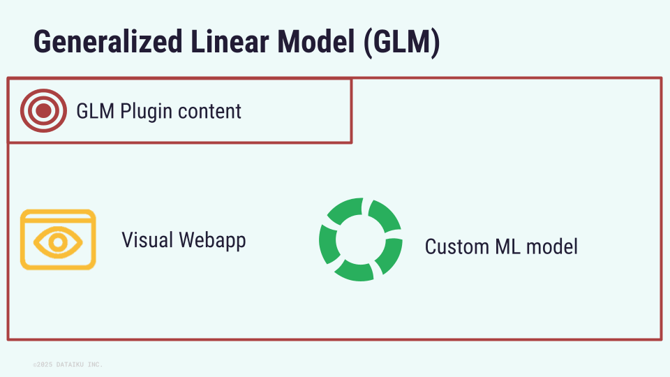
The GLM is available through a plugin. Not only does it introduce a GLM model in Visual ML as a custom model, but it also provides a full interactive experience to test and adjust models with its GLM visual webapp.
Business case: Car insurance#
GLMs are used in insurance and banking fields for pricing and credit scoring tasks. It is specifically indicated for claim modeling.
Use cases needing the GLM often involves an exposure variable. It is a known quantity that represents the amount of observation time, area, or population at risk. It adjusts for the fact that different observations may have had different opportunities for the event to occur. Depending on the predictor, the exposure variable may be different.
Let’s have a look to some relevant examples.
Claim frequency#
Claim frequency \(C_f\) is defined as the number of claims per year:
Where \(C_n\) is the number of reported claims for a given policyholder, and \(E\), the exposure, is the duration of the policy in years. When modeling the claim frequency, the goal is to predict the expected number of claims a policyholder will report in a year. Exposures can vary as customers did not all start their contract at the same time. So, normalizing by the exposure allows having comparable responses.
It is often modeled as a Poisson distribution.
Claim severity#
Claim severity \(C_s\) is defined as the claim amount per claim:
Where \(C_a\) is the total reported claim amounts for a given policyholder. Similarly to claim frequency, this normalization makes claim amounts comparable. This claim severity is only available when at least one claim has been reported by the policyholder.
It’s often modeled as a gamma distribution.
GLM visual webapp#
The GLM visual webapp is the core feature of the plugin. You just need to create it as any other visual webapp. This section presents the different tabs.
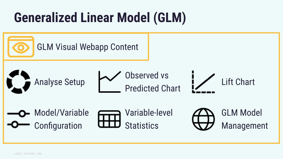
Analysis setup#
The Analysis Setup allows you to select a previously made analysis or create a new one from scratch.
Model and variable configuration#
The Model/Configuration tab of the webapp allows you to directly configure your GLM with core settings such as the distribution and link functions. You can also modify the different variables to include them as you see fit. Within this panel, you can define interactions between variables. The GLM webapp allows you to train the configured model without leaving the interface.
Observed vs. predicted chart#
The Observed vs Predicted Chart tab lets you visualize the observed and predicted values of the target variable with respect to a selected variable. The values can come from either the train or test dataset and you can compare different models. You can modify several settings such as the level order and the chart distribution.
Note
In this tab and next two, you can deploy the model.
Variable-level statistics#
The Variable-Level Statistics tab summarizes the statistics of the different numerical variables and categories of categorical variables from a given model. You can export these statistics.
Lift chart#
The Lift Chart tab allows you to create a lift chart for a given model. You can define the number of bins and choose which dataset (training or test) to use for the analysis. You can export the lift chart once created.
GLM model management#
The GLM Model Management table provides a quick overview of all GLMs created in your analysis. You can deploy, export, or delete them. Clicking on one of them opens an overview in the Visual ML tool.
Next steps#
GLMs allow actuaries to model phenomena that cannot be captured by simple linear regression. Also, they provide better control over variable dependencies compared with pure ML models. To see a GLM in action, you can explore the following: