
Concept | Generate features recipe#
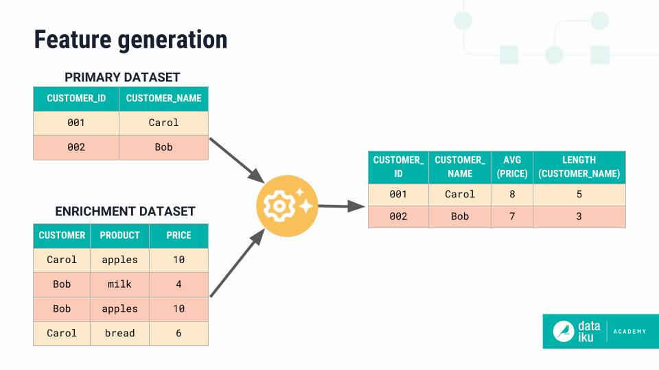
Data scientists often perform feature engineering, the process of creating new features from input datasets to improve model performance. Feature engineering can include transformations like numerical aggregations, extracting date parts, and computing values within certain time windows, among many other options.
One important consideration when performing feature engineering is to avoid introducing leakage, or generating features on future information that you would not know at prediction time, into your model.
Dataiku’s Generate features recipe allows discovering and generating many new features from your existing datasets, while avoiding prediction leakage, in one clean visual interface.
The recipe allows you to:
Configure relationships between a primary dataset and enrichment datasets.
Set associated time settings.
Select columns to compute new features on.
Perform transformations on them.
Important
See the reference documentation on the Generate features recipe for compatible dataset connections.
Data relationships#
The first step of building a feature generation recipe is to select your primary dataset, or the dataset you want to enrich with new features. Usually the primary dataset will contain a target variable whose values you want to predict.
The next step is to add enrichment datasets to compute new features on and ultimately enrich your primary dataset with. This step involves configuring:
Time settings#
There are a few key time settings that allow you to avoid introducing data leakage for machine learning problems and also to specify the time ranges you use in feature generation.
The cutoff time, which is set on the primary dataset, indicates the last point in time that data from enrichment datasets can be used for feature generation.
Caution
Setting a cutoff time has no effect unless you also set a time index on at least one enrichment dataset.
The time index of an enrichment dataset indicates when an event occurred corresponding to each row of data in that dataset.
Caution
If you set a time index on an enrichment dataset, all rows whose time index value is greater than or equal to the cutoff time will be excluded in feature generation.
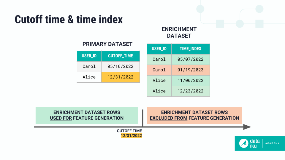
Let’s imagine we wanted to predict whether a user was going to make a purchase at a given time. Our primary dataset has a USER_ID column as well as a cutoff time column indicating when we’d want to make predictions by. Our enrichment dataset has a USER_ID column and a time index column corresponding to events that occurred.
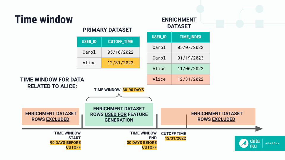
Time windows are based on the time index column and allow you to further narrow the time range used in feature generation. The example below for the user Alice shows a time window from 30 to 90 days before the cutoff time that would include 60 days of data from the enrichment dataset.
Join conditions and relationship types#
Also in the data relationships step, you need to determine how exactly to join your datasets. This includes selecting the join keys and relationship type based on the join keys.
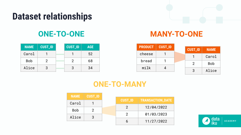
The relationship type can be:
One-to-one: One row in the left dataset matches one row in the right dataset.
One-to-many: One row in the left dataset matches many rows in the right dataset.
Many-to-one: Many rows in the left dataset match one row in the right dataset.
The relationship type informs how the recipe will generate new features. The recipe will compute row-by-row transformations — or, computations on one row at a time — on all datasets, regardless of the relationship type. But it will only perform aggregations — or, computations on many rows at once — on datasets that are on the right side of a one-to-many relationship. In these relationships, the join key will be used as the group key for aggregations.
Columns for computation#
After you’ve configured the data relationships, the next step is Columns for computation, where you select columns that you want to compute new features on. Note that for the primary dataset and any datasets with which the primary dataset has a one-to-one or many-to-one relationship, original values will also be retrieved for selected columns.
The variable type informs the types of transformations performed on selected columns. You can change the variable type to modify the types of transformations generated.
Feature transformations#
In the Feature transformations step, you can then choose the transformations you want to apply to selected columns for each variable type.
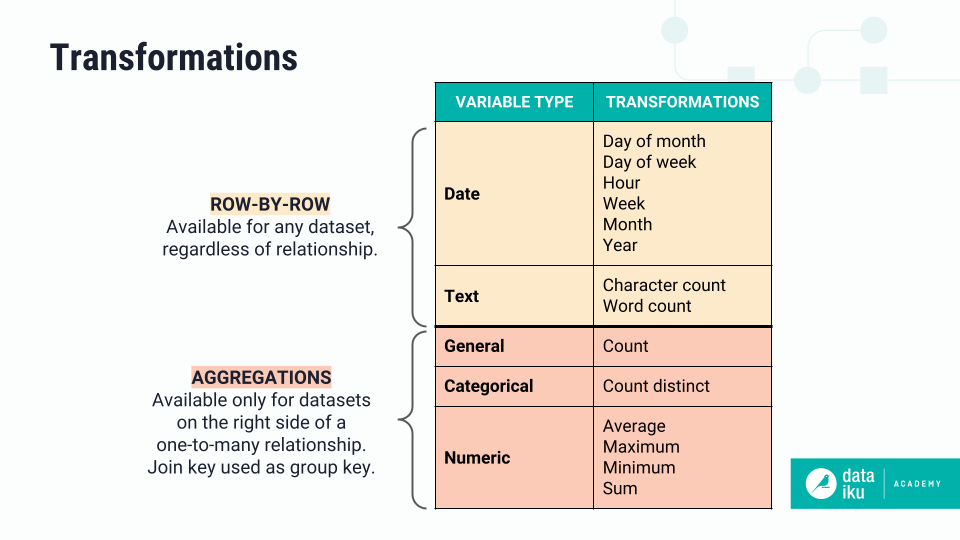
Feature transformations can either be:
Row-by-row: On date and text columns in all datasets, regardless of relationship type.
Aggregations: On general, categorical, and numerical columns, only on datasets that are on the right side of a one-to-many relationship. In these cases, the join key is used as the group key for aggregations.
The feature counter at the bottom left shows how many new columns the recipe will create. The counter changes as you select or deselect columns to compute or feature transformations.
Bringing it all together#
Let’s look at some examples to better understand how this recipe computes transformations for each relationship type.
One-to-one#

If the relationship is one-to-one the recipe will:
Join the datasets using the join conditions configured.
Perform selected row-by-row transformations on all date and text columns.
In this example, we join on the transaction_ID column, and compute transformations on the date column to find the month and year of each transaction date.
Many-to-one#

If the relationship is many-to-one, the recipe will:
Join the datasets using the join conditions you configured.
Perform selected row-by-row transformations on all selected date and text columns.
In this example, we join on the cust_ID again, and the recipe computes row-by-row transformations on the date.
You may have noticed that the steps are the same between many-to-one and one-to-one. These two relationship types actually perform the same computation under the hood!
One-to-many#

If the relationship is one-to-many, the recipe will:
Perform a group by on the join keys of the right dataset, and perform selected aggregations on all selected general, categorical, and numerical columns.
Join the datasets using the join conditions you configured.
Perform selected row-by-row transformations on all selected date and text columns.
In this example, we join on the cust_ID column, and compute aggregate transformations on the price, then row-by-row transformations on the name and birthdate.
In practice, the recipe begins by performing row-by-row computations on the outermost dataset, then follows the joins to the primary dataset
Note that another common use case for this recipe is self joins, or joining the same dataset onto itself, in order to generate interesting new features.
Output#
In the Output step, you can see the output column names, and even view the underlying query or convert it to an SQL recipe.
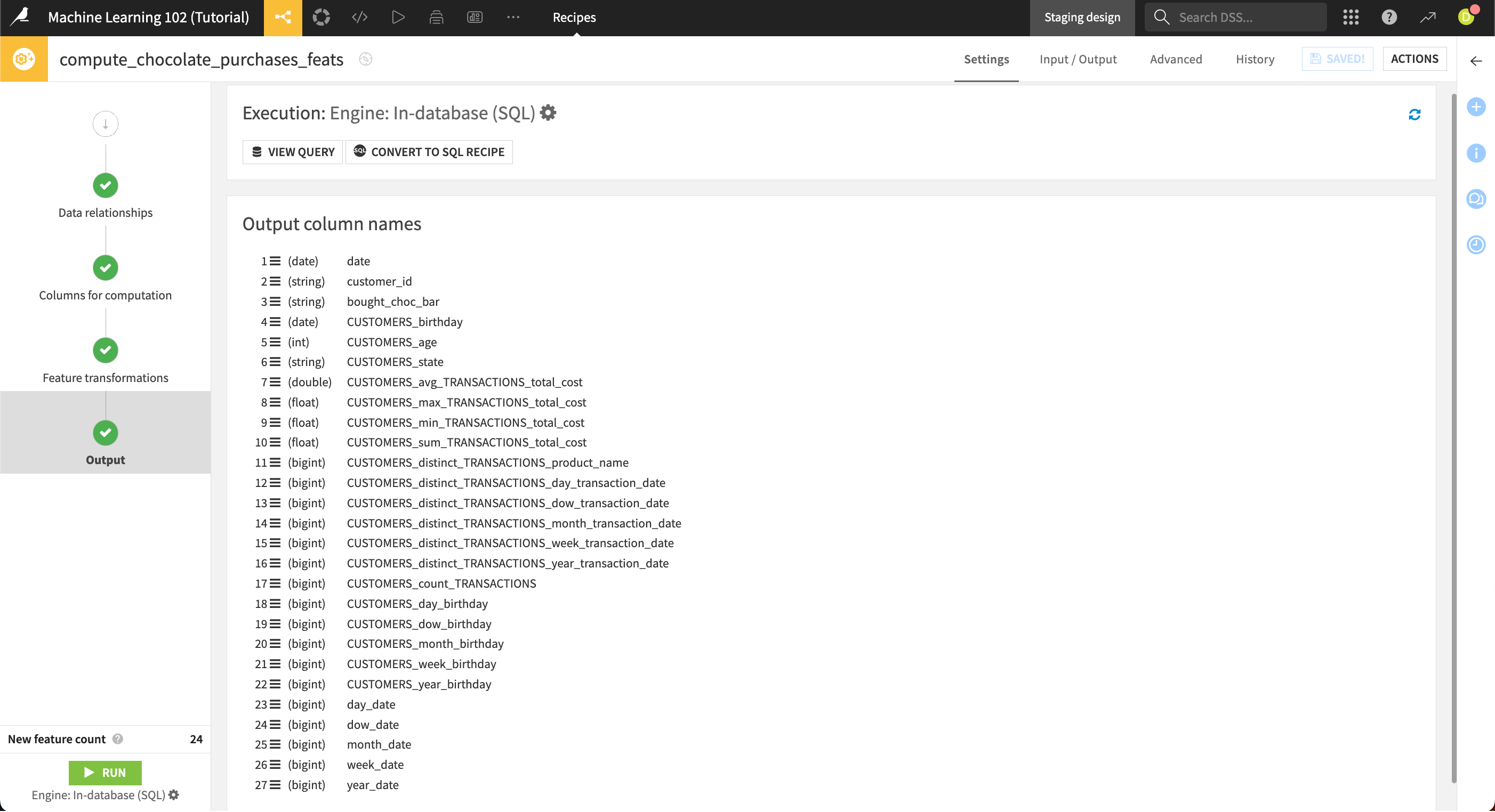
The output dataset contains column names and descriptions that show how the recipe computed each feature. The output column names include the original feature name and each of the transformations that take place on that feature.
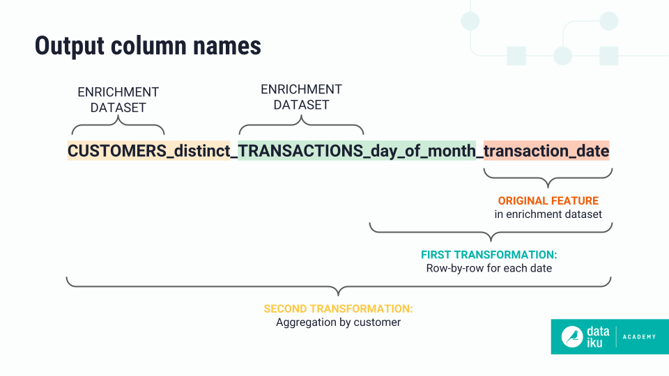
To help understand the output columns, it’s useful to know how the recipe works behind the scenes. Starting with the dataset that’s furthest from the primary, the recipe first performs row-by-row transformations on that dataset, and then moves iteratively toward the primary, performing computations based on relationship types. The column names reflect this iteration. In this example, there is a one-to-many relationship between the primary dataset and the secondary transactions dataset.
The number of features generated by this recipe can be quite large, and the transformations can become complex. For tips on how to reduce the number of features or complexity of transformations taking place, please see the reference documentation on the recipe to Generate features.
Any advanced feature reduction can be performed in the Lab once you train your model, as usual.
Next steps#
To see the Generate features recipe in action, complete Tutorial | Generate features recipe.