
Concept | Causal prediction#
Introducing causal prediction#
Most common data science projects using machine learning are centered around the idea of prediction. Such projects generate a model able to return a prediction over possible outcomes, given some inputs.
However, in many use cases, the ultimate goal shifts from purely predicting outcomes to optimizing such outcomes, given some actionable variables. For instance, instead of predicting which customers will most likely churn, businesses would rather focus their efforts on customers that will best respond to their actions (emails, discounts, etc.).
This is where causal prediction comes into play.
Causal prediction refers to the set of techniques used to model the incremental impact of an action or treatment on a given outcome. In other words, it’s used to investigate the causal effect of an action or treatment on some outcome of interest. For example, would patients recover faster if they get a specific treatment? Or would customers renew a subscription or churn if they receive a follow-up action (whether promotions, discounts, emails, or phone calls)?
The causal prediction analysis available in the Lab brings to Dataiku an out-of-the-box solution to train causal models and use them to score new data to predict the effect of some actionable variables, optimize interventions, and improve business outcomes.
To do so:
In the causal prediction analysis, we indicate one treatment variable (discount, ad, treatment in a clinical trial, etc.) along with a control value to tag rows where the treatment wasn’t received.
Upon training, the algorithm compares, for each observation, the observed outcome with the counterfactual outcome, namely, the predicted outcome under a different treatment value — and this is where machine learning is useful. Indeed, the counterfactual outcome has to be predicted as we can only observe one of the two potential outcomes. It’s impossible to observe someone’s reaction both when receiving the treatment and not receiving it.
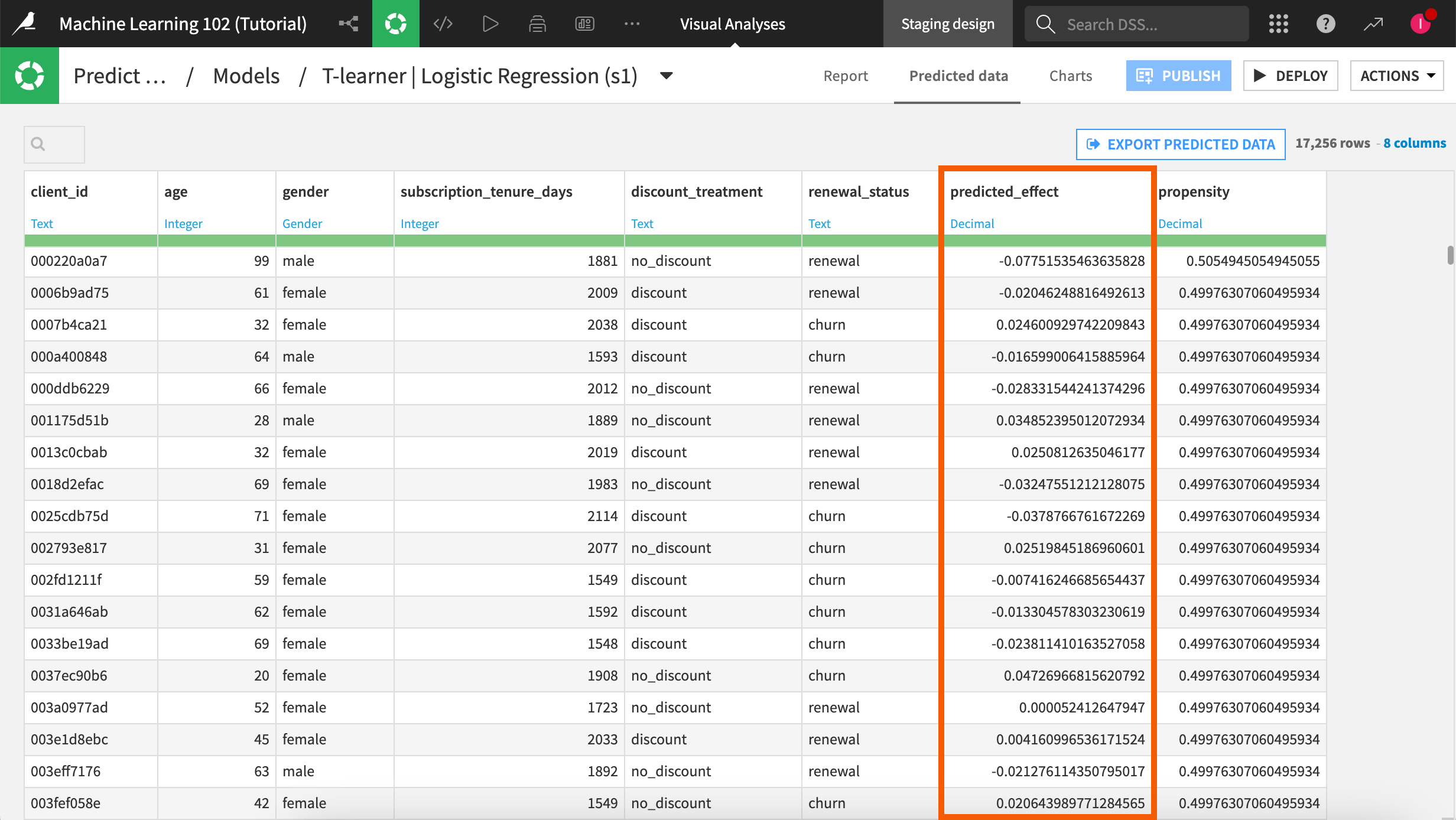
The model returns, for each row of the dataset, a treatment effect — that is, the difference between the outcomes with and without treatments, all else equal. This difference is often referred to as the individual treatment effect. It allows identifying who will “benefit” the most from the treatment to optimize treatment allocation.
A business use case: Uplift modeling to avoid customer churn#
A typical business use case is using causal prediction to prevent customer churn in B2Cs as customer retention is key to profitability.
It’s important to target the customers who react positively to an action to avoid a waste of time and money.
To know how a given customer would react to a follow-up action, they need to know whether that customer would renew when they get treated with a marketing action (T = 1) as well as when they remain untreated (T = 0). In other words, for a given customer, we’re interested in measuring the Individual Treatment Effect (ITE) or Causal Effect defined as:
Where:
Yi(Ti) stands for the potential outcome of individual i under treatment Ti.
Yi(1) is thus an indicator for subscription renewal when i receives the treatment.
Yi(0) the same outcome when i doesn’t receive it.
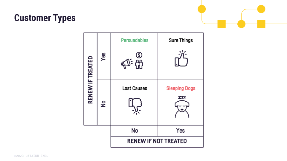
The combinations of those different potential outcomes give rise to four customer types:
Sure Things: These customers will renew with and without treatment: τi = 1 - 1 = 0
Lost Causes: These customers will churn with and without treatment: τi = 0 - 0 = 0
Sleeping Dogs: These customers will churn if treated and renew if not treated: τi = 0 - 1 = -1
Persuadables: These customers will renew if treated and churn if not treated: τi = 1 - 0 = 1
In the case of customer churn, causal prediction is used to make predictions about the effect of the treatment on the renewal outcome at the individual level to ultimately focus on targeting only the Persuadables subpopulation.
With a good causal model and this customer segmentation in mind:
Persuadable customers should have a predicted Conditional Average Treatment Effect (CATE) approaching 1.
Sleeping Dogs should have their prediction approach -1.
Sure Things and Lost Causes should have a predicted CATE close to 0.
Note
The CATE is the average treatment effect for a subgroup in the population.
Note that for qualitative metrics, you should refer to the AUUC and Qini curves available in the Causal Performance section of the model’s Report tab.
The importance of assumptions#
With causal prediction, the identification and estimation of causal effects rely on crucial assumptions about the data. Assumptions can help to guide the selection of variables that are likely to be predictive of the treatment effect and to ensure that the modeling approach is appropriate to answer your question.
Unsatisfied assumptions may result in errors in the predictions and misguide business decision-makers.
In this section, we’ll introduce some key assumptions, namely ignorability and positivity.
Ignorability (aka unconfoundedness)#
Ignorability means that the treatment assignment is independent of the potential outcomes realized under treatment or control. In other words, there should be no unmeasured confounders that may affect the relationship between the treatment and the outcome. All the covariates affecting both the treatment variable and the outcome variable are measured and can be used in the causal model to estimate the causal effect of the treatment.
For example, let’s say we have an education case where we want to see the effect of the college degree (the treatment). If an unobserved covariate (such as the student ability) is positively correlated with both the treatment variable (college degree) and the outcome variable (salary), the causal effect of the treatment on the outcome variable will be biased (that is, the treatment effect isn’t identified).
Another example is when a medical treatment is more readily given to people with a lower, unmeasured chance of recovery. The treatment effect on recovery will be biased downwards. Another identifiability failure example is when a business offers discount vouchers only to their customers that are more likely to generate more revenue with the voucher. Here, we would simply overestimate the effect of the discount.
With randomized trials, we can ensure that the treatment and control groups aren’t assigned in a biased way, relative to any covariates that can impact the outcome. So both the treatments and controls should include people in each gender, each predisposition, etc. If a covariate is unbalanced (more females than males in a gender covariate for instance), it might be better to remove the covariate from the analysis to avoid bias.
Randomization means that each individual is given a 50% chance of receiving the treatment.
Enabling the treatment analysis in Dataiku (Modeling > Treatment analysis panel within the Design tab of the causal prediction analysis) helps assess whether the randomization is violated. It returns some metrics in the Treatment analysis > Treatment randomization panel of the model’s Result page after training.
Note
For more information, see Treatment randomization in the reference documentation.
Positivity (aka common support)#
The positivity assumption ensures that every observation has a non-zero probability of being in the treatment group or control group (that is, strictly greater than 0 and less than 1).
A violation of this assumption means that for a subset of the data, either everyone receives the treatment or everyone receives the control. In either case, we’re missing a comparison group and causal models will need to extrapolate CATE predictions from the predictions of not-so-similar units. This is an estimability issue.
This propensity isn’t known and needs to be estimated. To do so, Dataiku offers to build a propensity model (Modeling > Treatment analysis panel within the Design tab of the causal prediction analysis), which is of paramount importance for two reasons:
First, it’s the basis for checking whether the positivity assumption holds and potentially identifying violating subpopulations in the data. Once those subpopulations are identified, we may try to fix the common support assumption using two common strategies:
The first way is to simply recognize that CATE predictions for those subpopulations are extrapolated (read unreliable) and need to be discarded.
The second option is to remove features from our analysis, if possible (say if they fully characterize the violating subpopulation). Unfortunately, this last strategy elevates the risk of introducing omitted variable biases in the CATE estimates. As we remove features, we may indeed remove confounders.
Note
The more features we use, the finer our data can be segmented into subpopulations. This inevitably increases the chances of picking up a violation of the positivity assumption in some of those finer subpopulations.
Second, some classes of causal models rely on propensity score estimates to provide more robust predictions. Any errors in those estimates may compound into the CATE estimates.
Causal prediction metrics#
Always bear in mind that evaluation metrics used in causal prediction don’t measure a model’s ability to predict the outcome, such as churn. Instead,they measure the model’s ability to predict the treatment effect on the outcome**.
As there is no way of observing counterfactuals and thus knowing for sure what would have occurred if an individual had not received treatment (or vice versa), conventional evaluation metrics such as AUC can’t be used to assess causal models and specific metrics like the Area Under the Uplift and Qini curves are used.
Dataiku uses the following common metrics:
AUUC
Qini score, and
Net uplift
Area Under the Uplift Curve (AUUC)#
AUUC (Area Under the Uplift Curve) measures the percentage of total uplift that’s achieved by targeting a certain percentage of the population. This metric is useful for evaluating the effectiveness of targeting strategies and for comparing the performance of different models.
Note
This metric was created in the context of uplift modeling, a popular application of causal inference, hence its name. Yet, the AUUC can be used to assess the predictions of any causal model no matter the use case for which it’s used.
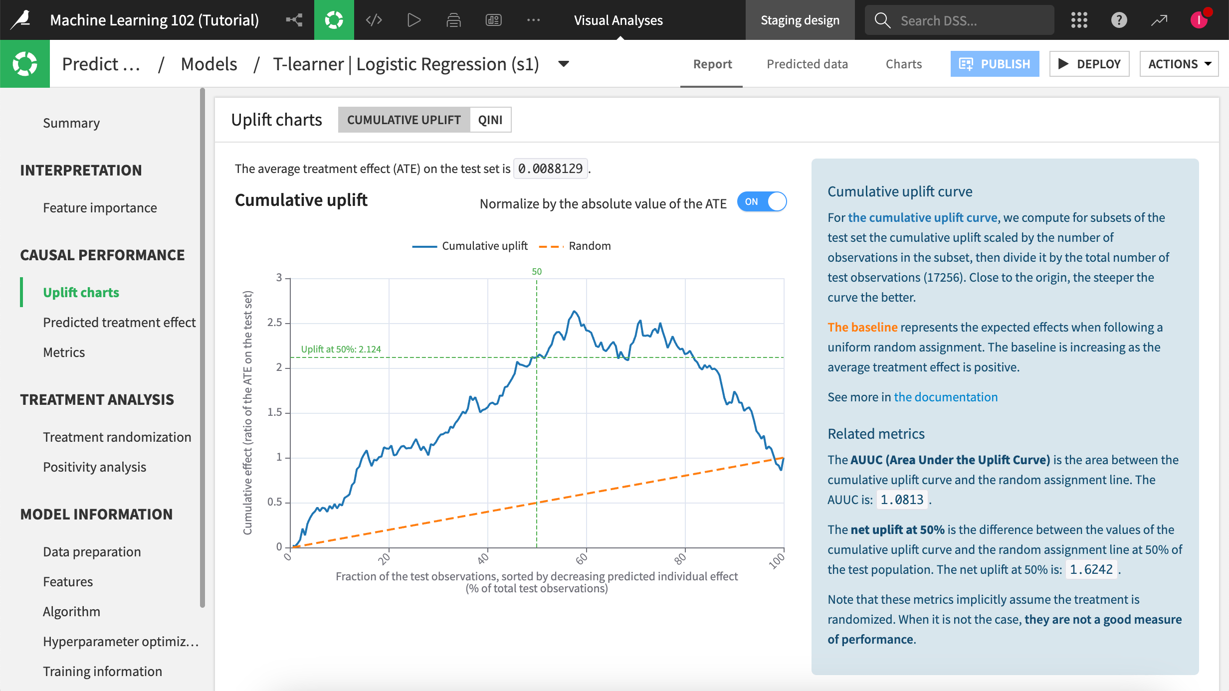
The screenshot above shows an example of an uplift curve and a baseline corresponding to the global treatment effect on the test data. The positive slope of this baseline line means that the treatment has an overall positive effect on the sample. A bell-shaped uplift curve indicates that the uplift model is good — high uplift predictions correspond to a large difference in average outcome. The declining portion of the curve shows the negative effect of treatment and should be located to the right of the curve as we include samples with lowest predicted uplift.
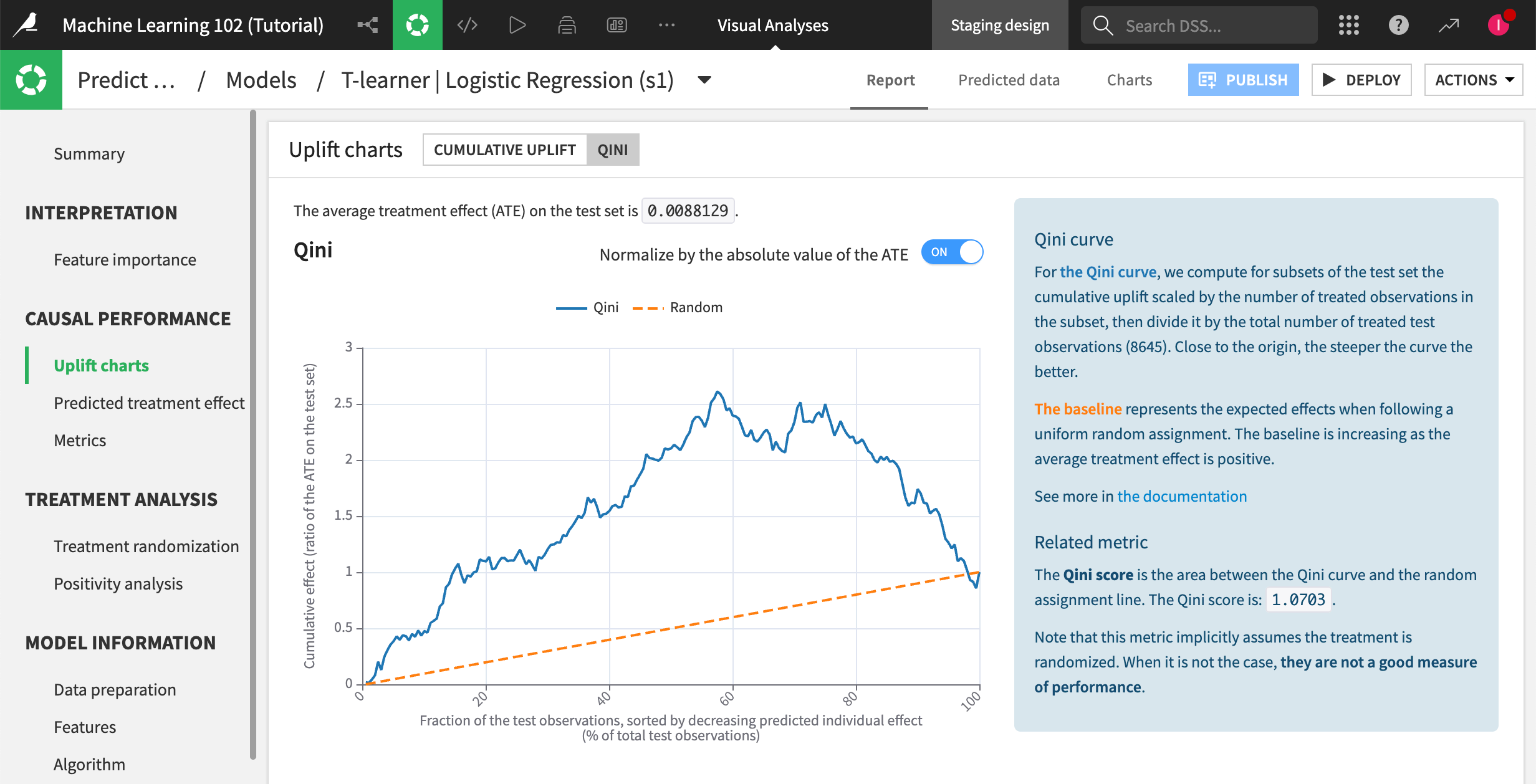
Qini score#
Qini curves are another useful tool for evaluating the performance of uplift models. A Qini curve plots the cumulative uplift against the cumulative proportion of the population targeted. The steeper the curve, the more effective the model is at identifying the subgroups of individuals who are most likely to benefit from the treatment.
Net uplift#
Net uplift measures the difference in the expected outcome between the treatment and the control groups, after accounting for the cost of the treatment. This metric is useful for evaluating the profitability of an action and for making decisions about resource allocation.
The net uplift at 50% is the difference between the values of the cumulative uplift curve and the random assignment line at 50% of the test population.