Tutorial | Model scoring basics#
Get started#
In the machine learning basics tutorial, we trained a model to predict the “high revenue potential” of customers for whom we’ve already observed their previous long-term behavior.
Before we can use this model to generate predictions, we’ll need to add it to the Flow.
Objectives#
In this tutorial, you will:
Deploy the best performing model from the Lab to the Flow so that it can be used for scoring new data.
Use the Score recipe to apply a predictive model to new data.
Prerequisites#
Dataiku 12.0 or later.
Basic knowledge of Dataiku (Core Designer level or equivalent).
You may also want to review this tutorial’s associated concept article.
Create the project#
From the Dataiku Design homepage, click + New Project.
Select Learning projects.
Search for and select Scoring Basics.
If needed, change the folder into which the project will be installed, and click Create.
From the project homepage, click Go to Flow (or type
g+f).
Note
You can also download the starter project from this website and import it as a ZIP file.
Tip
Alternatively, you can continue working in the project you created in the Machine Learning Basics tutorial.
You’ll next want to build the Flow.
Click Flow Actions at the bottom right of the Flow.
Click Build all.
Keep the default settings and click Build.
Use case summary#
This tutorial uses a classification model trained on historical customer records and order logs from a fictional company, Haiku T-Shirts. We will apply the model to a new, unlabeled dataset to predict whether new customers are expected to be of high revenue potential.
Deploy the model#
Our Flow has a customers_labeled dataset used to train a predictive model. We also have some new customers (the customers_unlabeled_prepared dataset) for whom we have the first purchase, and we want to predict whether they’ll turn out to be high revenue customers.
Return to the model in the Lab#
First, you’ll need to return to the model in the Lab.
Open the High revenue analysis attached to the customers_labeled dataset. You can do this by clicking on the dataset and going to the Right panel > Lab > High revenue analysis. You can also use the keyboard shortcut
g+a.While looking at the Result tab, open the model report for the best performing Random forest model by clicking on its name.
We’re choosing to deploy this particular model because it has the best performance of the trained models for this project. In practice, model selection depends on a number of factors, which could include simplicity, interpretability, limiting bias, and so on.
Tip
You can document your best models to allow others to find and understand them more easily. From the main Result view, you can “star” a model to note its importance. When you dive into the individual summary of a model, you can edit the model name and give it a description.
Deploy the model to the Flow#
We’re now going to deploy this model to the Flow, where we’ll be able to use it to score another dataset.
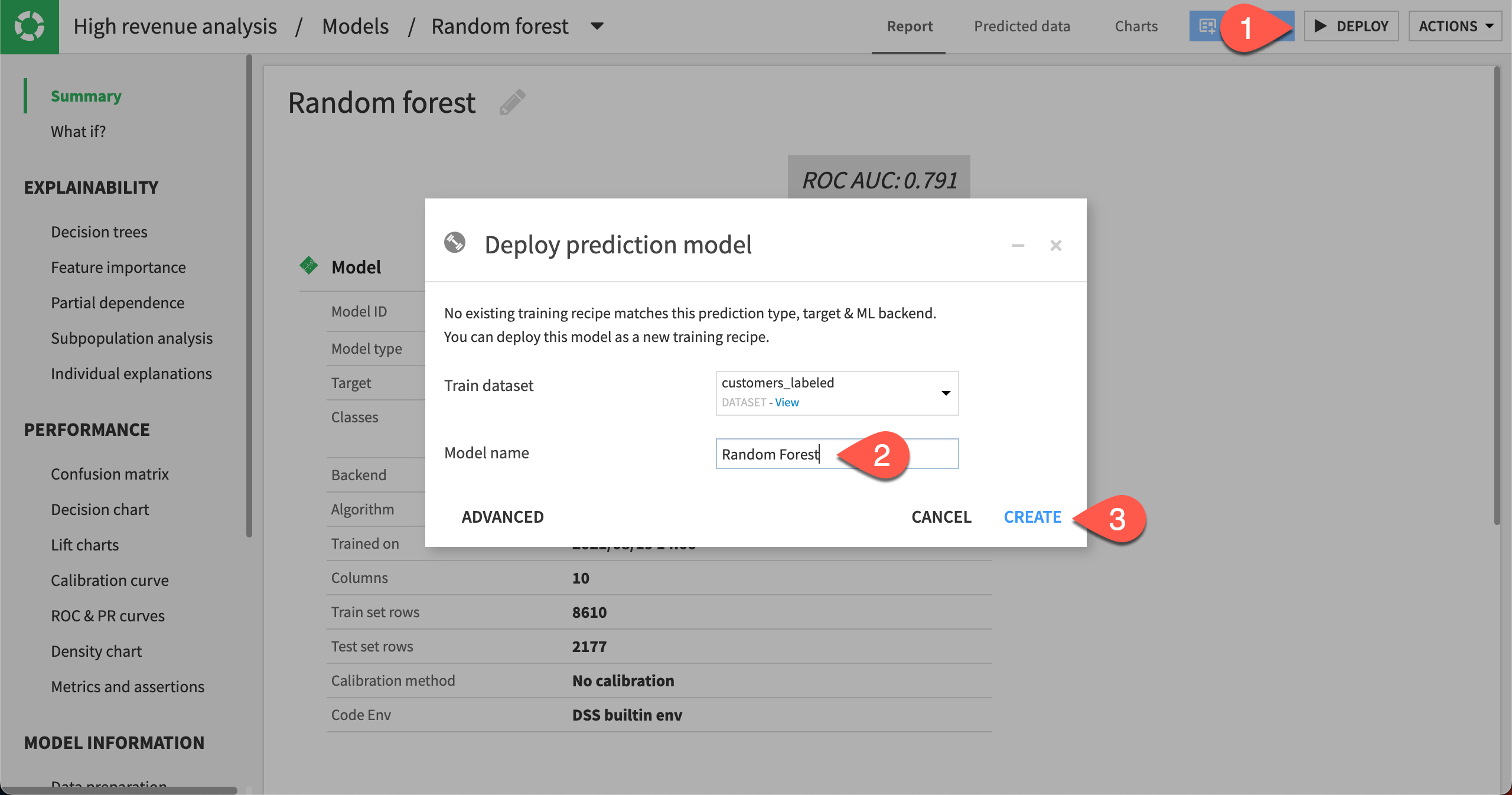
While viewing the model report, click on the Deploy button near the top right.
In the dialog, change the Model name to a more manageable
Random Forest.Click Create.
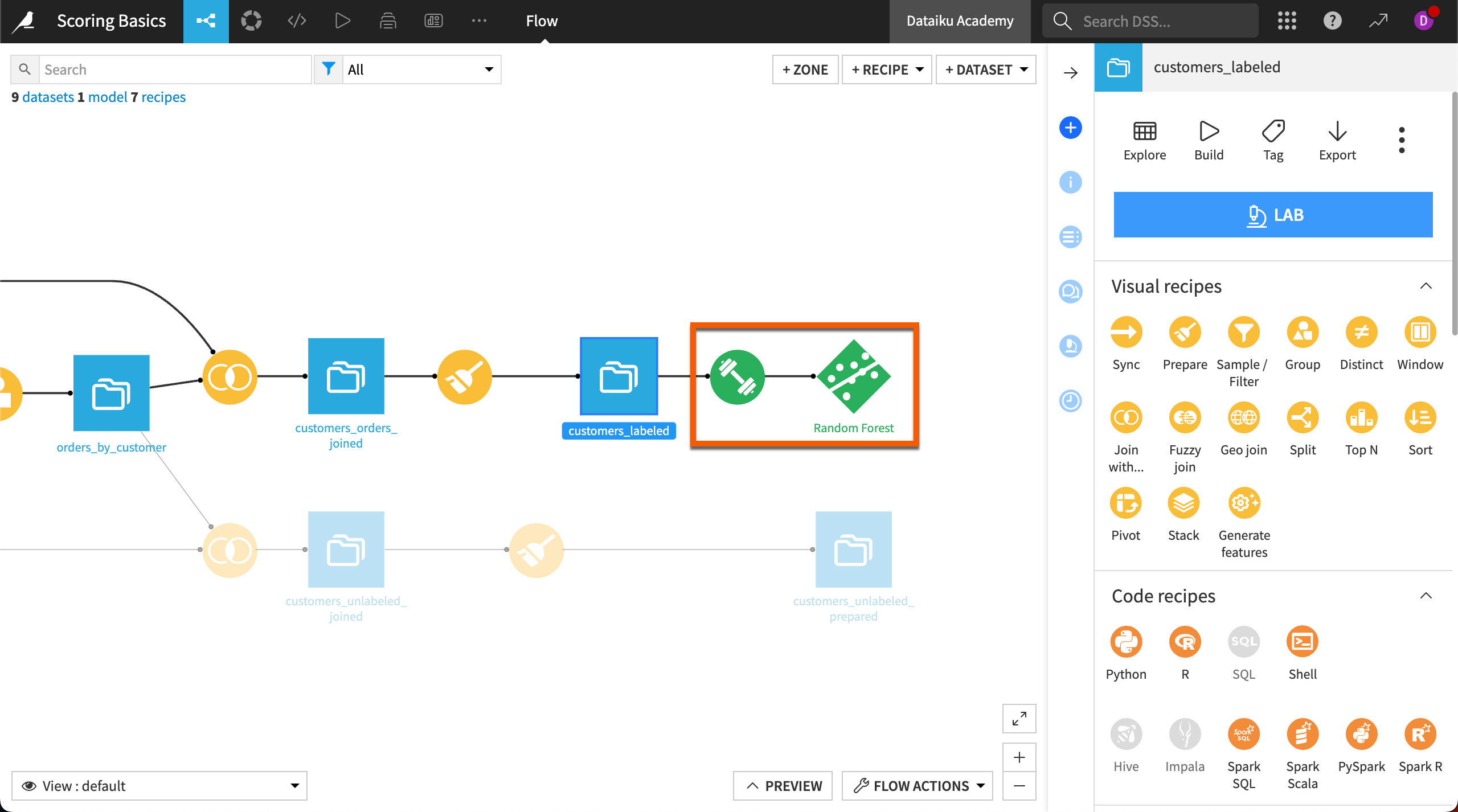
You will now be taken back to the Flow where two new objects with green icons have been added:
The first one is the Train recipe, which is the way to deploy a model to the Flow where you can use it to produce predictions on new records.
The second new object is the Train recipe output, the saved model.
Score new data#
We can now use the deployed model in the Flow to make predictions about new customers. First, we’ll double check the model and our data to be scored.
Check the active version of the model#
Let’s take a closer look at the saved model object.
From the project’s Flow, double click to open the Random Forest model.
Notice that the model is marked as the Active version.
If your data were to evolve over time (which is likely in real life!), you could train your model again by selecting Actions and then Retrain in the Actions panel. In this case, new versions of the models would be available, and you would be able to select which version of the model you’d like to use.

Check the schema of the data to be scored#
Let’s confirm that the schema of the data we plan to score has the same features as the training data.
Return to the Flow.
Select the customers_unlabeled_prepared dataset.
Open the Schema (
) tab in the right panel.
Compare it with that of customers_labeled.
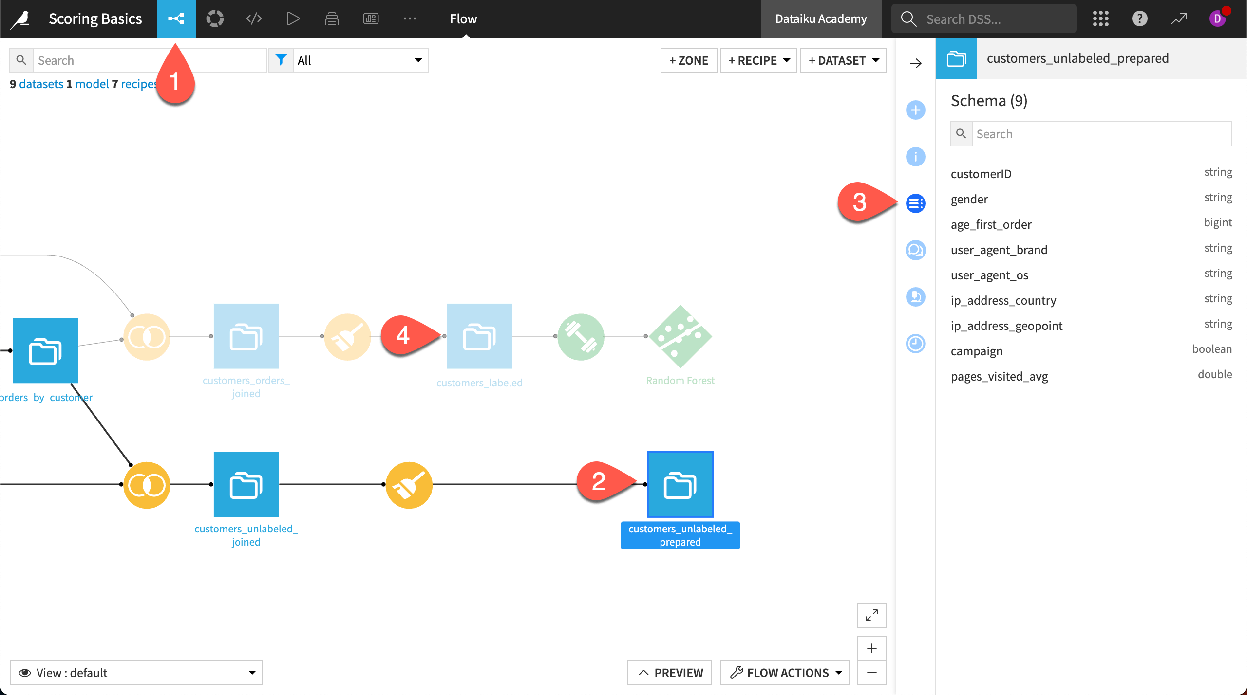
You can see that customers_unlabeled_prepared has the exact same features as customers_labeled. The only difference is that customers_unlabeled_prepared is missing the high_revenue column, which is the target variable that the model will predict.
Create a Score recipe#
Having confirmed the same features are available, we’re ready to apply the model to new data.
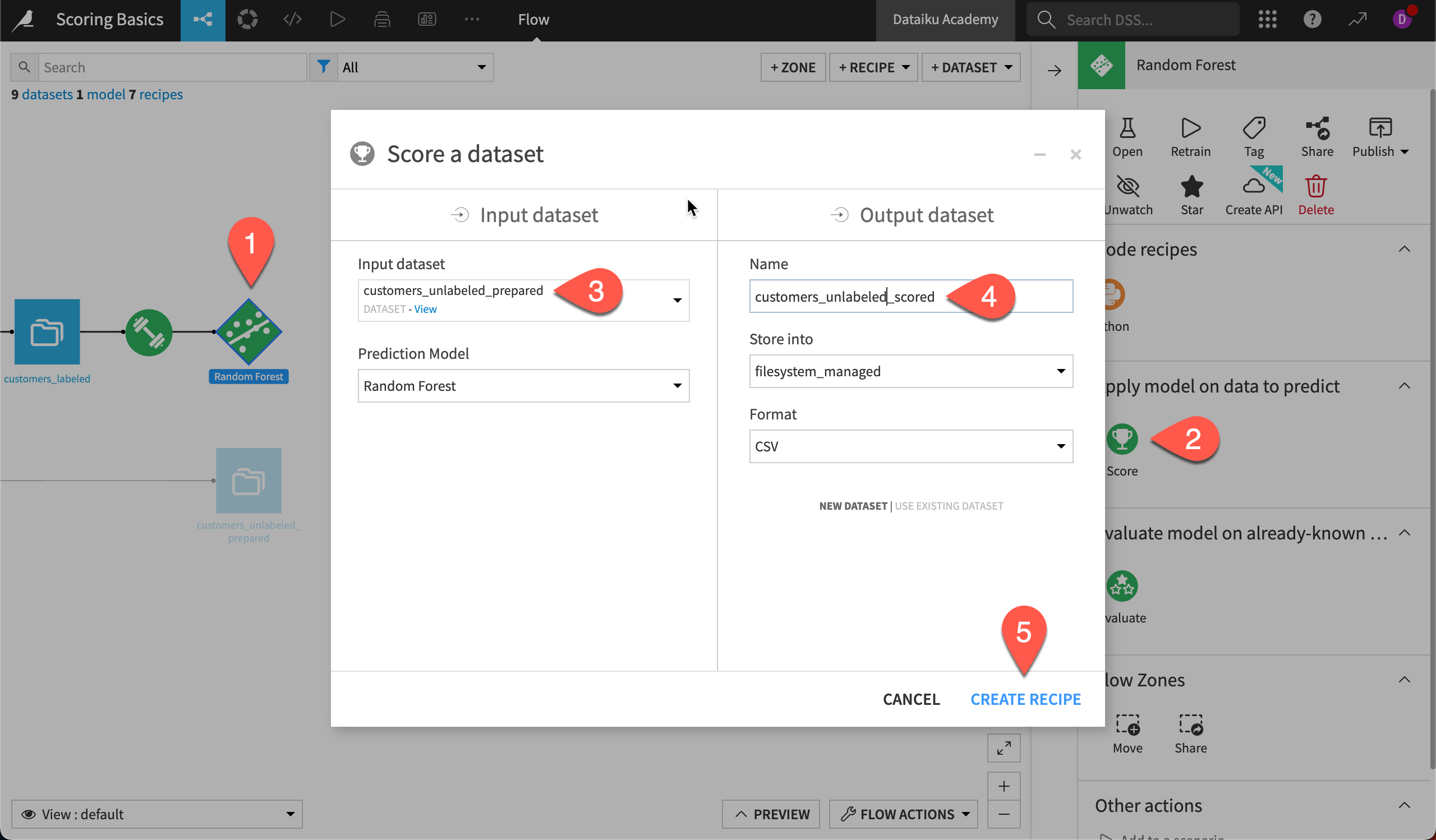
Select the deployed model Random Forest in the Flow.
Choose the Score recipe from the right panel.
In the dialog, set the Input dataset to customers_unlabeled_prepared.
Name the Output dataset
customers_unlabeled_scored.Click Create Recipe.
Note
In this case, we selected the model first, and so found the Score recipe in the Actions panel. If we had selected the dataset for scoring first instead of the model, we would find a Predict recipe in the Actions panel. Regardless of whether you select the model first or the dataset first, these are both the same Score recipe!
Configure a Score recipe#
There are a few options to consider when configuring a Score recipe.
The threshold is the optimal value computed to maximize a given metric. In our case, it was set to 0.625. Rows with probability values above the threshold will be classified as high value, below as low value.
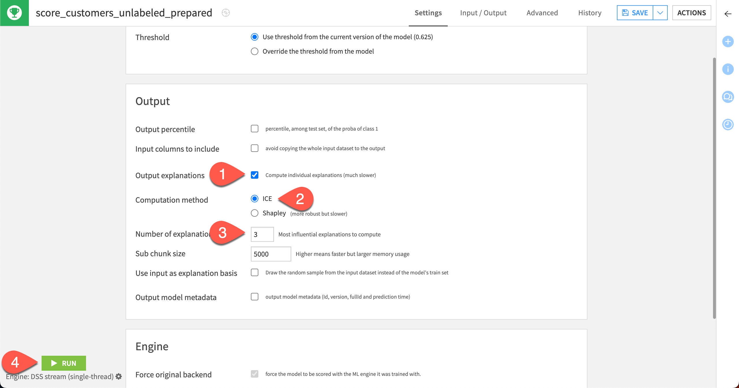
If you would like to return individual explanations of the prediction for each row in the customers_unlabeled_prepared dataset:
Select the Output explanations checkbox, which will enable some additional parameters below.
For the Computation method, keep the default ICE.
For the Number of explanations, keep the default
3. This returns the contributions of the three most influential features for each row.Select the Run button to score the dataset.
Back in the Flow, you’ll be able to see your progress.
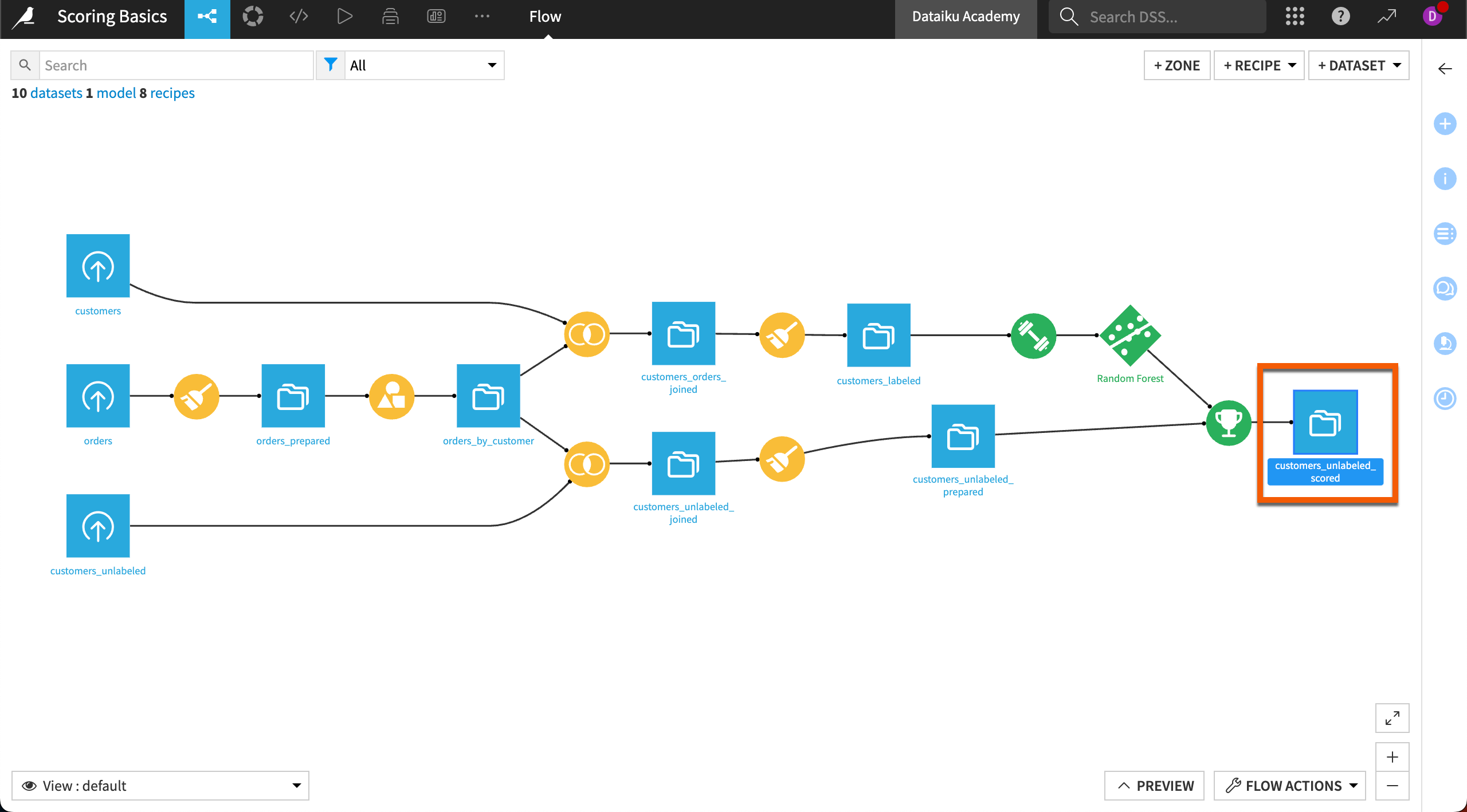
Inspect the scored results#
We’re almost done!
Open the customers_unlabeled_scored dataset to see how the scored results compare to the recipe input or the training data.
Four new columns have been added to the dataset:
proba_False
proba_True
prediction
explanations (as requested in the Score recipe)
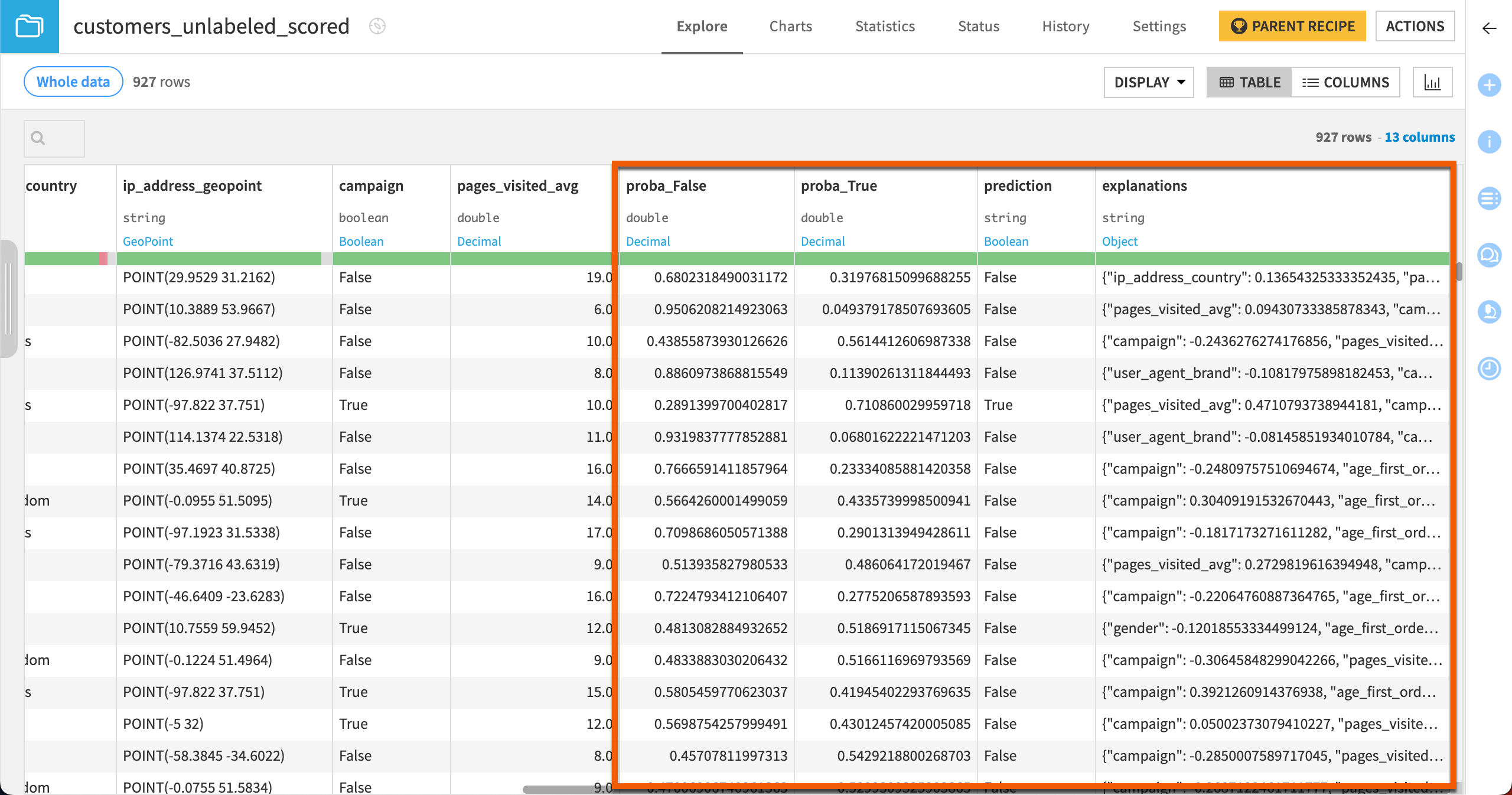
The two proba_ columns are of particular interest. The model provides two probabilities, that is, a value between 0 and 1, measuring:
how likely a customer is to become a high value customer (proba_True),
how likely a customer will not become a high value customer (proba_False).
The prediction column is the decision based on the probability and the threshold value of the Score recipe. Whenever the column proba_True is above the threshold value (in this case, 0.625), then Dataiku will label that prediction as True.
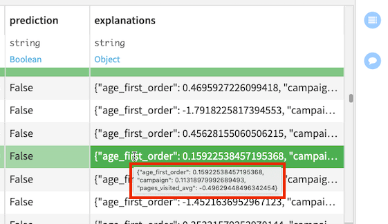
The explanations column contains a JSON object with features as keys and their positive or negative influences as values. For example, the highlighted row in the following figure shows the three most influential features (age_first_order, campaign, and pages_visited_avg) for this row and their corresponding contributions to the prediction outcome.
Unnest JSON data (optional)#
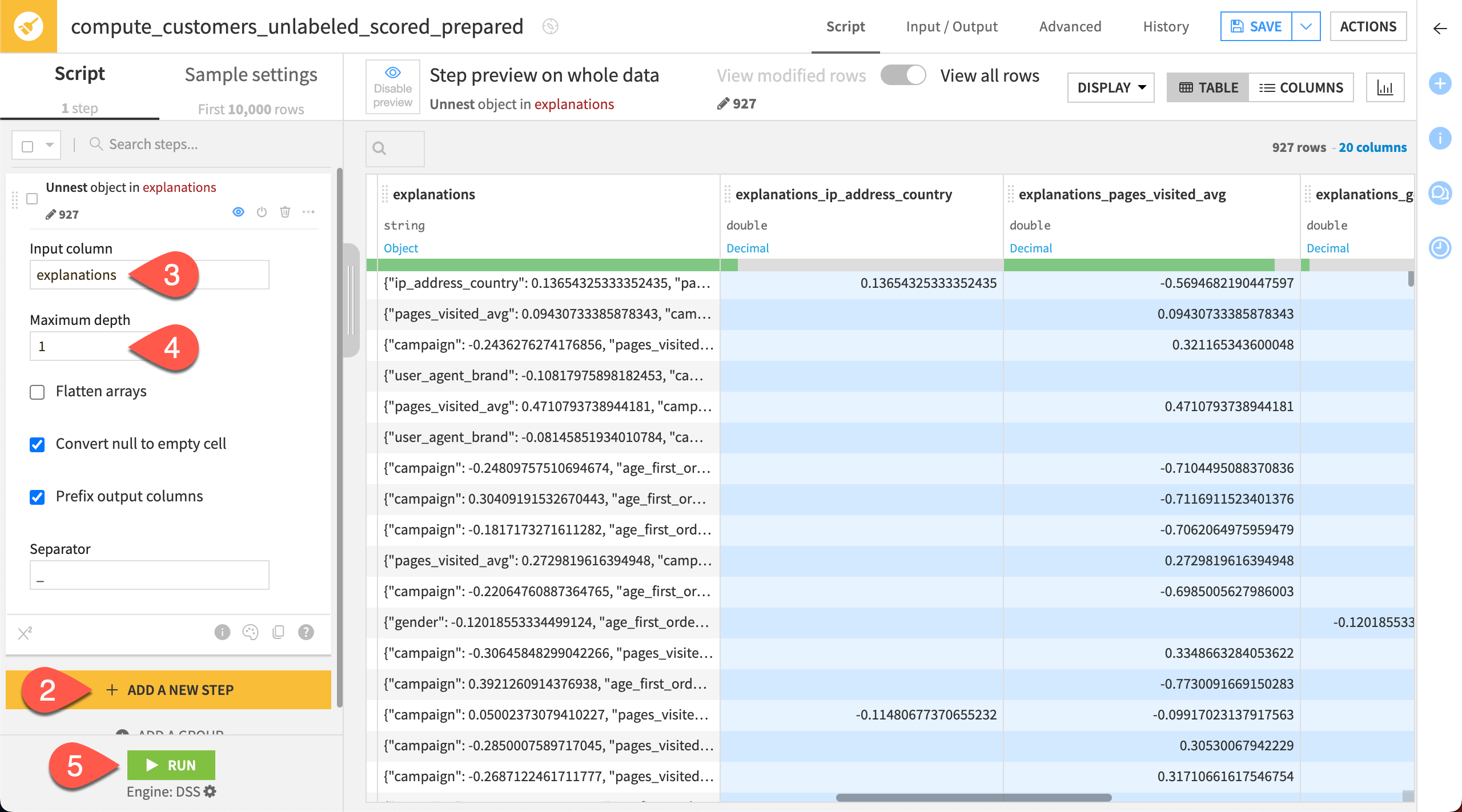
We can more easily work with the JSON data in the explanations column after using the Prepare recipe.
Create a Prepare recipe with customers_unlabeled_scored as the input dataset.
Click + Add New Step, and choose Unnest object.
Choose explanations as the input column.
Set the maximum depth to
1.Click Run.
See also
Learn more about Individual prediction explanations in the reference documentation.
Next steps#
Congratulations! You have deployed a model to the Flow and used it to make predictions on unlabeled data.
Your next step might be to challenge yourself to earn the ML Practitioner certificate.

