Concept | Time series fundamentals#

Introduction to time series#

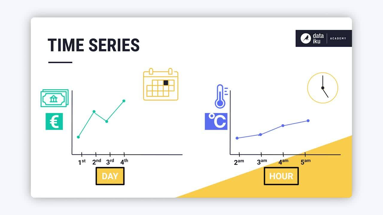
Time series data sets consist of repeated numerical measurements of a variable or entity ordered sequentially with time. Data sets containing variables such as the daily closing prices of a stock, or repeated measurements of the average hourly temperature of a room are examples of time series.

Time series properties#

Some properties of time series include:

Time series property	Description
Time dependence	As in the previous examples, the variables in a time series depend on time.
Chronological ordering	The values in a time series are ordered in sequence.
Equispaced values	Time series data entries arrive in equally spaced time intervals, such as hourly, daily, yearly, and so on. In addition, raw time series data can sometimes contain irregularly spaced entries, thereby requiring some processing to space the data equally.

The time interval used for collecting time series data can depend on data availability and the analysis to be performed on the dataset. For example, data on your electricity usage may be available on the hourly level.

However, if you want to study the evolution of your monthly electricity usage, it would be more appropriate to collect this data monthly. Various resampling techniques are available for converting your data from one time interval level to another.

Because of the properties mentioned earlier, time series data sets are different from other tabular data sets that are typically used in data analysis (for example, a dataset containing measurements of wine density recorded at a specific time).

Time series use cases#

Use cases of time series can be found in a wide range of industries, such as:

Field	Example
Economics	Describe the quarterly GDP growth of a country.
Meteorology	Forecast the average monthly temperature of a region.
Advertising	Predict the weekly number of page views for a website.
Finance	Analyze the daily price changes of stocks.

Time series data types and formats#

This article covers the different types of time series datasets and the formats in which they can be stored.

Types of time series data#

A time series dataset can contain one or more variables of an entity repeatedly measured over time. Depending on the number of variables in a time series, and the relationships between the variables, time series data can be categorized as:

Univariate
Multivariate
Multiple

Univariate#

A univariate time series consists of sequential measurements of a single variable over time.

Consider a time series dataset that contains measurements of a person named Mike, who has certain features (or variables), such as gender, height, weight, and pulse. If we collect measurements of one of these variables, say Mike’s weight, over time, we have a univariate time series.

Important

Using these values of Mike’s weight, we can build a model to predict his future weight.

Multivariate#

A multivariate time series consists of sequential measurements of multiple related variables over time.

For example, suppose our data set consists of the measurements of Mike’s height and weight, and we know that there is a relationship between the two variables (weight and height). In that case, we have a multivariate time series. Or, more specifically, a bivariate time series. This is because our dataset consists of exactly two variables that are interrelated.

Important

Using these values of Mike’s weight and height, we can build a prediction model to determine his future weight or height.

Multiple#

A time series data set is said to contain multiple time series if it contains measurements of multiple entities that are independent.

Now, let’s build upon the univariate example by including measurements of Kate’s weight. Suppose we know that the measurements of these individuals are independent of each other.

In that case, we can say that the dataset contains multiple univariate time series, and predicting the weight of an individual would depend on his or her previous weights alone.

Furthermore, if the dataset also contains the heights of these two individuals, then we have multiple multivariate time series in our dataset.

Time series data formats#

Dataiku works with time series datasets that come in wide format or long format.

Wide format#

To explain the wide format, consider the case where the time series dataset consists of multiple univariate time series-—-the weights for Mike and Kate. This dataset is in wide format if each univariate time series is stored in a separate column.

Furthermore, the dataset could contain multiple multivariate time series. Such as the measurements of Mike’s height and weight (a multivariate time series) and the measurements of Kate’s height and weight (another multivariate time series).

Wide format representation is easy to understand and more natural to use when plotting. However, using this format can present issues when there are missing values in the data. For example, if Mike decides to drop out of this experiment, we must decide whether to keep adding empty rows for Mike’s measurements.

Or whether to drop Mike’s columns entirely.

Long format#

This format provides a compact way of representing multiple time series. Consider a time series dataset that consists of multiple univariate time series. In long format, values from the univariate time series are all stored in the same column.

Storing the data this way makes it necessary to have an identifier column that tells us which time series each row belongs to.

A multivariate time series dataset can also be stored in long format, and in this case, the identifier column will list the variables of a given entity.

Using the long format can provide a more compact way to represent time series datasets when compared to the wide format. For illustration, consider that we have the weights for Mike and Kate, and we decide to start measuring Jon’s weight as well. Using long format, we would simply add a new row for Jon. Whereas, if our dataset is in wide format, we would have to add a new column for Jon, and fill in missing values for the dates before we made Jon’s first measurement.

Long vs. wide format#

Often, the choice of which format to use in storing time series data sets depends on the kinds of models that will be used on them.

For example, the wide format may be more suitable for analyses like MANOVA and repeated measures ANOVA. On the other hand, if we’re interested in mixed models or survival analysis, using long format may be more appropriate.

Time series components#

We can decompose a time series into four parts. These are:

Trend
Seasonality
Cycle
Random variation

Trend#

The trend is a non-repeating, long-term direction of a time series. Trends can be upward, downward, horizontal, linear, or nonlinear.

For example, see the upward and downward trend in the plot of Japan’s population.

Seasonality#

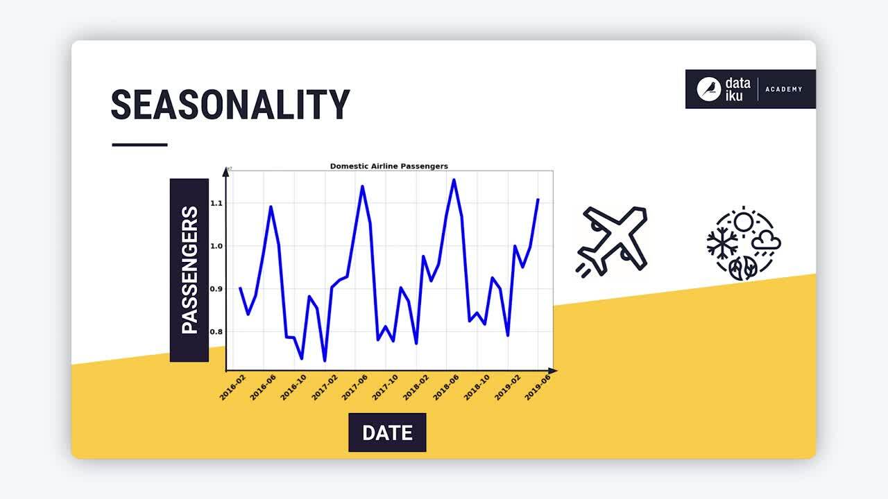
The seasonality describes a repeated behavior that occurs, over the short term, at predictable intervals that span less than a year.

Man-made events, such as airline travel, can lead to seasonality in data. Also, natural forces, such as weather and changing seasons, can cause seasonality, as is the case with crop production and sales of umbrellas.

Cycle#

Cycles occur when a time series follows a non-seasonal, up-and-down pattern. Cycles are hard to predict because they don’t occur in predictable time intervals.

A typical example is the business cycle, comprising the phases of recovery, prosperity, recession, and depression.

Seasonality vs. cycle#

Note these critical distinctions between seasonality and cycle.

When the changes in a time series repeat with a fixed frequency associated with some aspect of the calendar, then the changes are seasonal. Whereas, if the changes occur with varying frequencies, then they’re cyclical.
In general, the average length of cycles tends to be longer than that of seasonal patterns, and the magnitudes of cycles tend to be more variable than that of seasonal ones.

Random variation#

A random variation in time series data occurs due to uncontrollable and unpredictable events, such as earthquakes, wars, floods, famines, and so on.

This plot of the Nikkei 225 stock index shows a plunge in value, which coincided with the earthquake and tsunami in March 2011.

Modeling with time series components#

Identifying time series components is useful for understanding the underlying patterns in the data, and for modeling the data as a combination of the components.

Models can be additive, representing the time series as a sum of the components. Here, the magnitude of the seasonality tends to stay constant over time.
Models can also be multiplicative, representing the time series as a product of the components. In this case, the magnitude of the seasonality tends to increase over time.

Objectives of time series analysis#

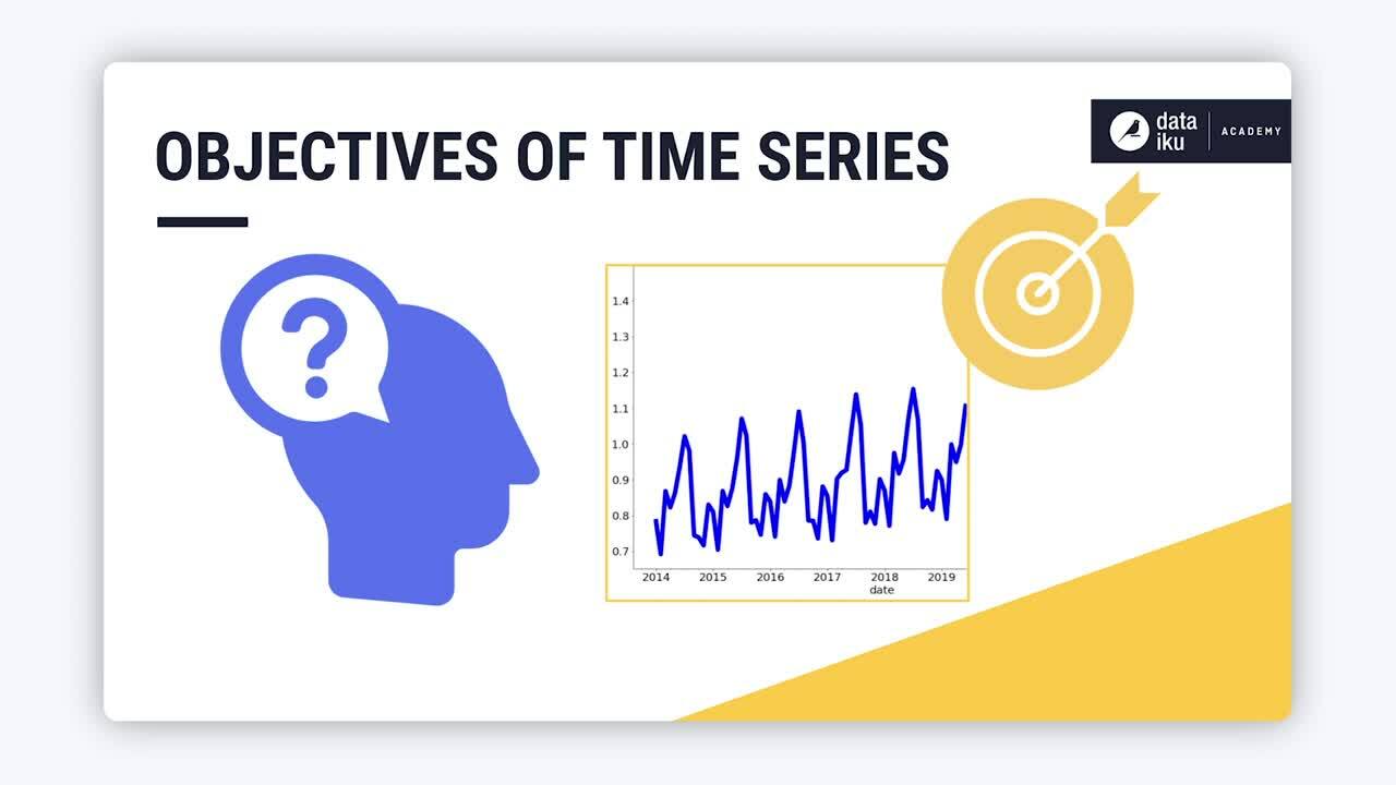
Knowing the objectives of a time series analysis is essential for choosing the right kinds of strategies to implement. Objectives can be:

Descriptive
Explanatory
Forecasting
Control

Descriptive#

A descriptive analysis is best served by plotting the time series data. Plotting provides a “high level“ overview of the time series and its main components: the trend, seasonality, cycle, and random variations.

For example, by plotting data on the number of domestic airline passengers in the United States from the U.S. International Air Passenger and Freight Statistics Report, we observe a seasonal pattern and an upward trend in the number of passengers over the years.

Plotting can also reveal any points in the data that appear inconsistent with the data pattern, that is, outliers.

Additionally, plotting can reveal turning points in the data, which can be useful when deciding on forecasting strategies. For instance, we may have to fit different models to portions of the data that occur before and after turning points.

Explanatory#

Suppose we want to explain the behavior of a multivariate time series data. We can use the changes in one variable to explain another variable, and thereby understand how the two variables are related.

Additionally, we can explain the behavior of a time series by training models on its components.

Forecasting#

Forecasting uses the observed values of a time series with a model to predict future time series values.

Several forecasting techniques are available for use with time series data. One example is the ARIMA model, which we’ve used with the airline dataset here to forecast the number of passengers for the upcoming years.

Control#

The goal of an analysis can also be to control a physical system or business outcome.

For example, an airline company may want to increase its profit by increasing the number of passengers who travel in a given period. Suppose a forecast of passengers shows a decline in travel for the said period. The airline may attempt to control this outcome by offering lower ticket prices or airline rewards, which could lead to an increase in its profit.