
Tutorial | Generate features recipe#
Get started#
Dataiku’s Generate features recipe makes it possible to discover and generate new features from your existing datasets for use in machine learning models. The recipe’s time settings also allow you to avoid leakage, or future information that you would not know at prediction time, into your models.
Tip
It’s useful to review the Concept | Generate features recipe article before following this tutorial.
Objectives#
In this tutorial, you will learn how to:
Use this recipe to configure relationships between a primary dataset and enrichment datasets.
Set associated time settings.
Select columns to compute new features on.
Perform transformations on them.
Prerequisites#
The Generate features recipe is available only for SQL datasets in Dataiku version 12.0, with additional support for Spark-compatible datasets in version 12.1. To follow along and reproduce the tutorial steps, you will need access to the following:
Dataiku 12.0 or later.
An SQL connection from the list of compatible connections.
Tip
If you don’t already have your own instance of Dataiku with an SQL connection, you can start a free Dataiku Cloud Trial from Snowflake Marketplace. This trial gives you access to an instance of Dataiku Cloud with a Snowflake connection.
Create the project#
From the Dataiku Design homepage, click + New Project.
Select Learning projects.
Search for and select Generate Features Recipe.
If needed, change the folder into which the project will be installed, and click Create.
From the project homepage, click Go to Flow (or type
g+f).
Note
You can also download the starter project from this website and import it as a ZIP file.
Exploration and connections#
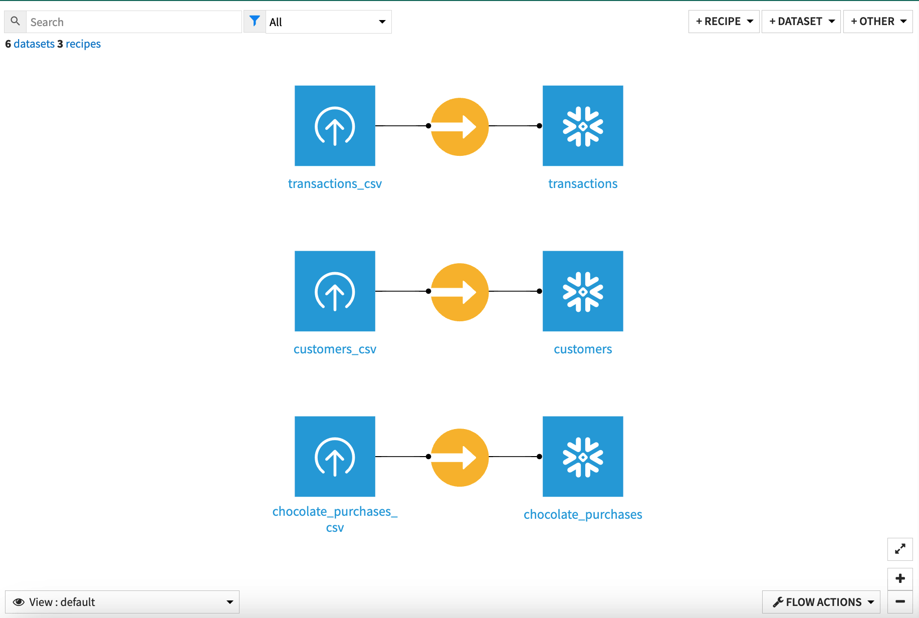
We’ll start with three small datasets illustrating a retail store’s customer database.
Explore each dataset and note the features of each. This fictional store tracks its customers, transactions, and the dates when each customer bought chocolate bars. Let’s say this store wants to build a machine learning model to predict which customers are likely to buy chocolate bars, in order to improve its email marketing. We’ll use these three basic datasets to generate some new features that could be used to build an even more robust model.
Note
The Generate features recipe requires dates to be parsed into standard format. The dates in our datasets have already been parsed, but in cases where they’re not, you would need to run Prepare recipes to parse the dates before using the Generate features recipe.
The recipe also requires that datasets are stored on connections that are compatible with SQL or Spark engines. So we’ll start by converting the datasets, which were imported from CSV files, into a supported dataset format.
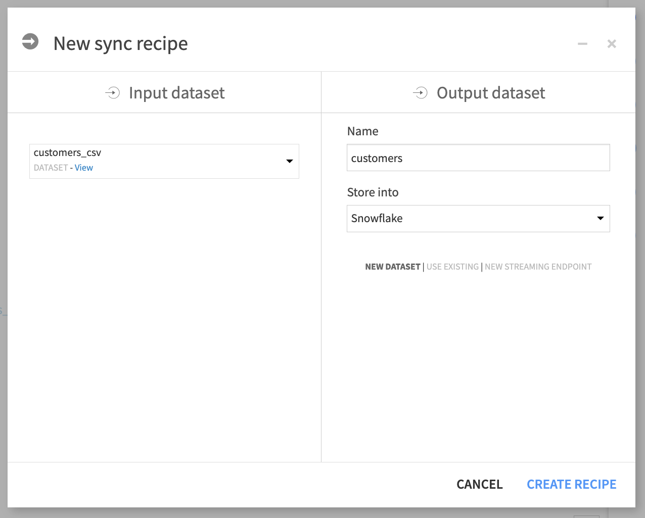
Highlight the customers_csv dataset.
In the right Actions panel, select the Sync recipe.
In the recipe creation info window, remove the _csv_copy extension from the output dataset name so that it’s named customers.
Store the dataset on your SQL or Spark-compatible connection. If you are using the Dataiku Cloud Trial from the Snowflake Marketplace, select the Snowflake connection. This tutorial will use Snowflake.
Click Create recipe.
In the recipe configuration window, click Run.
Repeat these steps for the other two datasets: transactions_csv and chocolate_purchases_csv.
With our datasets remapped to SQL connections, we’re ready to use the Generate features recipe.
Configure data relationships#
The Generate features recipe allows you to define relationships between a primary dataset, which you want to enrich with new features, and enrichment datasets, which will be used to compute new features. The primary dataset usually contains a target column whose values want to predict using a model.
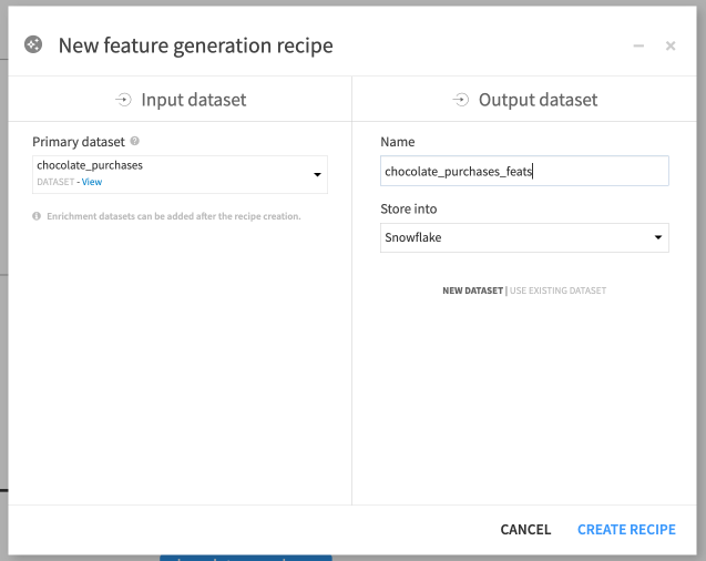
For this example, we want to predict whether the customer will buy a chocolate bar, so we’ll use chocolate_purchases as the primary dataset.
Highlight the chocolate_purchases dataset.
In the Actions panel on the right, select the Generate features recipe.
Rename the output dataset or keep the default name, chocolate_purchases_feats.
Store the output dataset on the same database connection as your input, and click Create recipe.
The recipe opens to the Data relationships tab, where we can configure join settings between the primary and enrichment datasets, define the relationship types, and set time conditions to prevent leakage in our model.
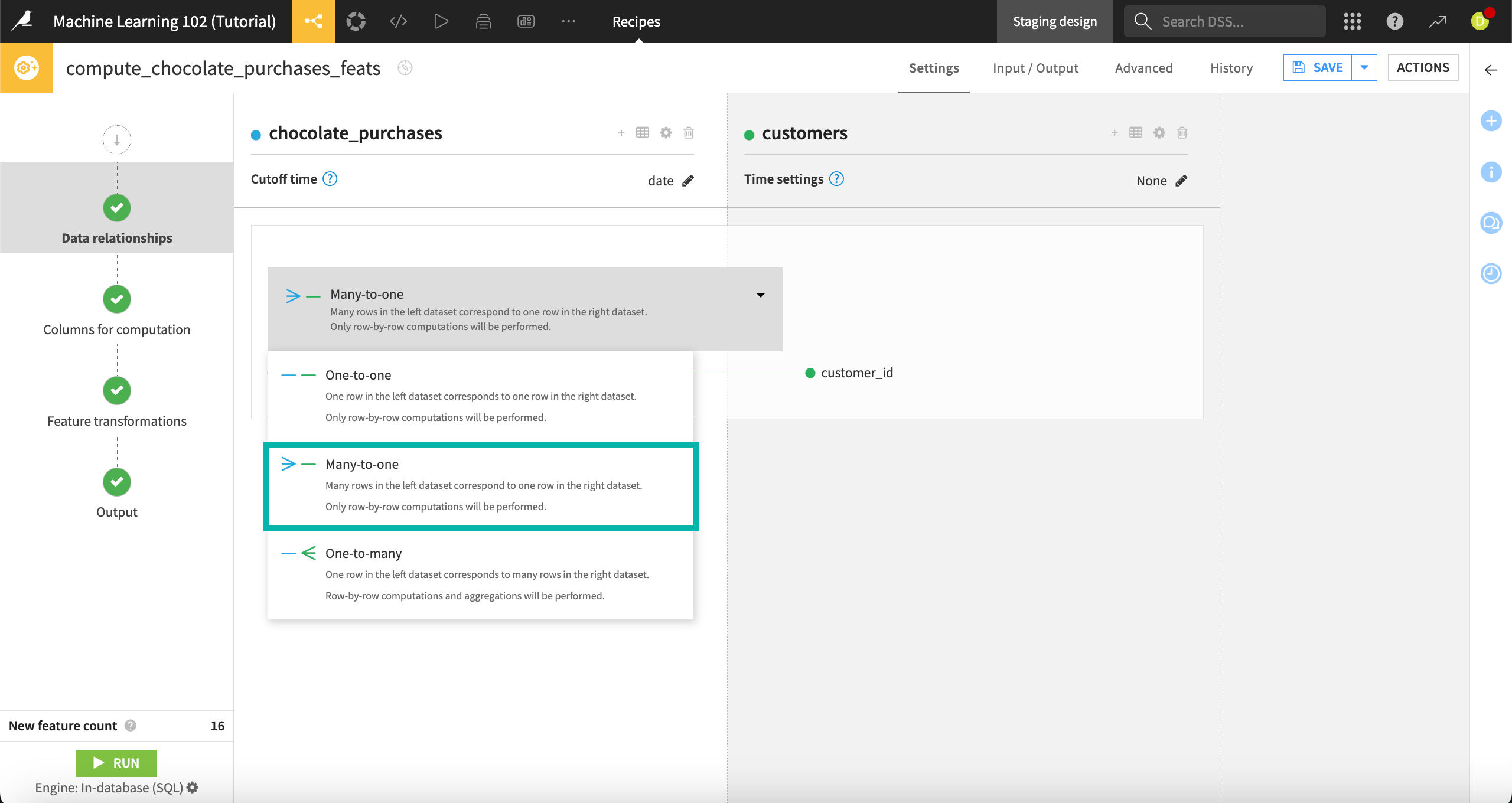
To add our first enrichment dataset, customers, we’ll need to know the relationship types and cutoff time. The chocolate_purchases dataset has a many-to-one relationship with customers, because there can be many chocolate bar purchases in the chocolate_purchases dataset for each customer in the customers dataset. Chocolate_purchases also includes a date column that we’ll use as a cutoff time.
For the cutoff time to impact the recipe’s computations, we’ll also need to set a time index on enrichment datasets, pointing to a column that indicates when an event associated with each row of data took place. That will ensure that any rows in enrichment datasets that take place after the primary dataset’s cutoff time are excluded from calculations. The cutoff time and time index together will prevent the recipe from introducing leakage, or generating features on future information that we would not know at prediction time, into our model.
To add customers as an enrichment dataset:
Select + Add Enrichment Dataset.
For the Cutoff time, select Date column. The date column will be autoselected, as it’s the only date column.
Under Enrichment dataset, choose the customers dataset as our first enrichment dataset.
For Time index, choose None. The customers dataset does have a date column, birthday, but this column doesn’t make sense to use as a time index, as we would not want to exclude customers from feature generation based on their birthdays.
Click Save, and return to the recipe settings.
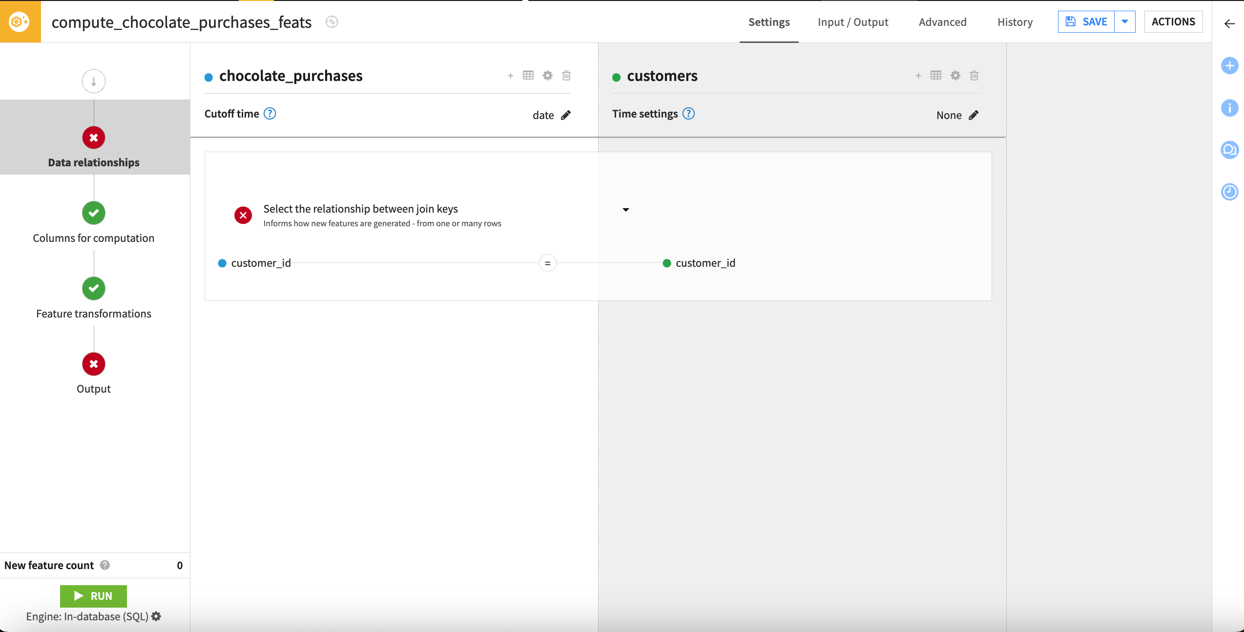
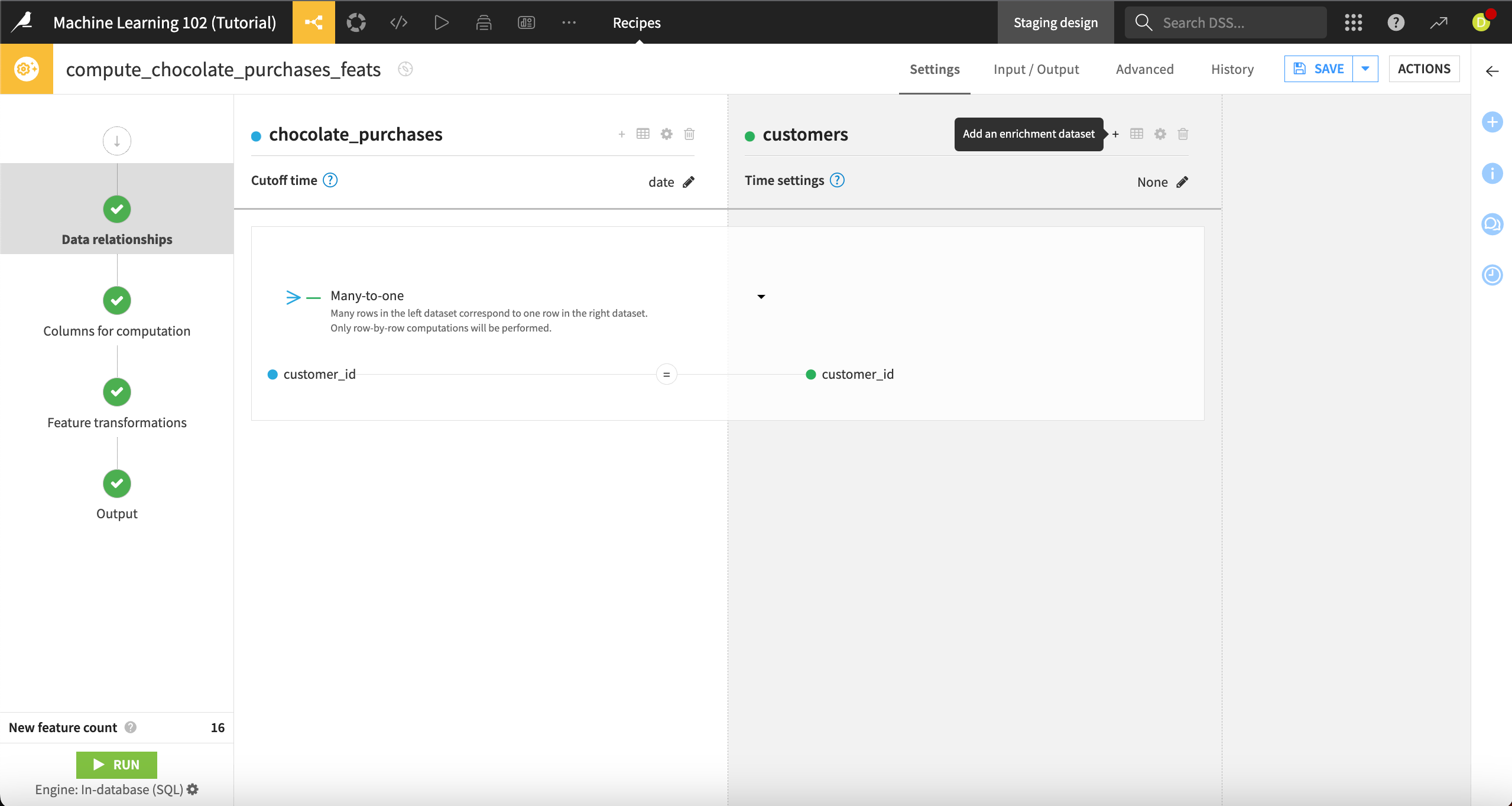
The recipe has automatically selected customer_id as the join key for these two datasets. We can leave this default selection untouched. We now need to select the relationship type between the datasets, based on the join keys.
Click on Select the relationship between join keys.
Select Many-to-one.
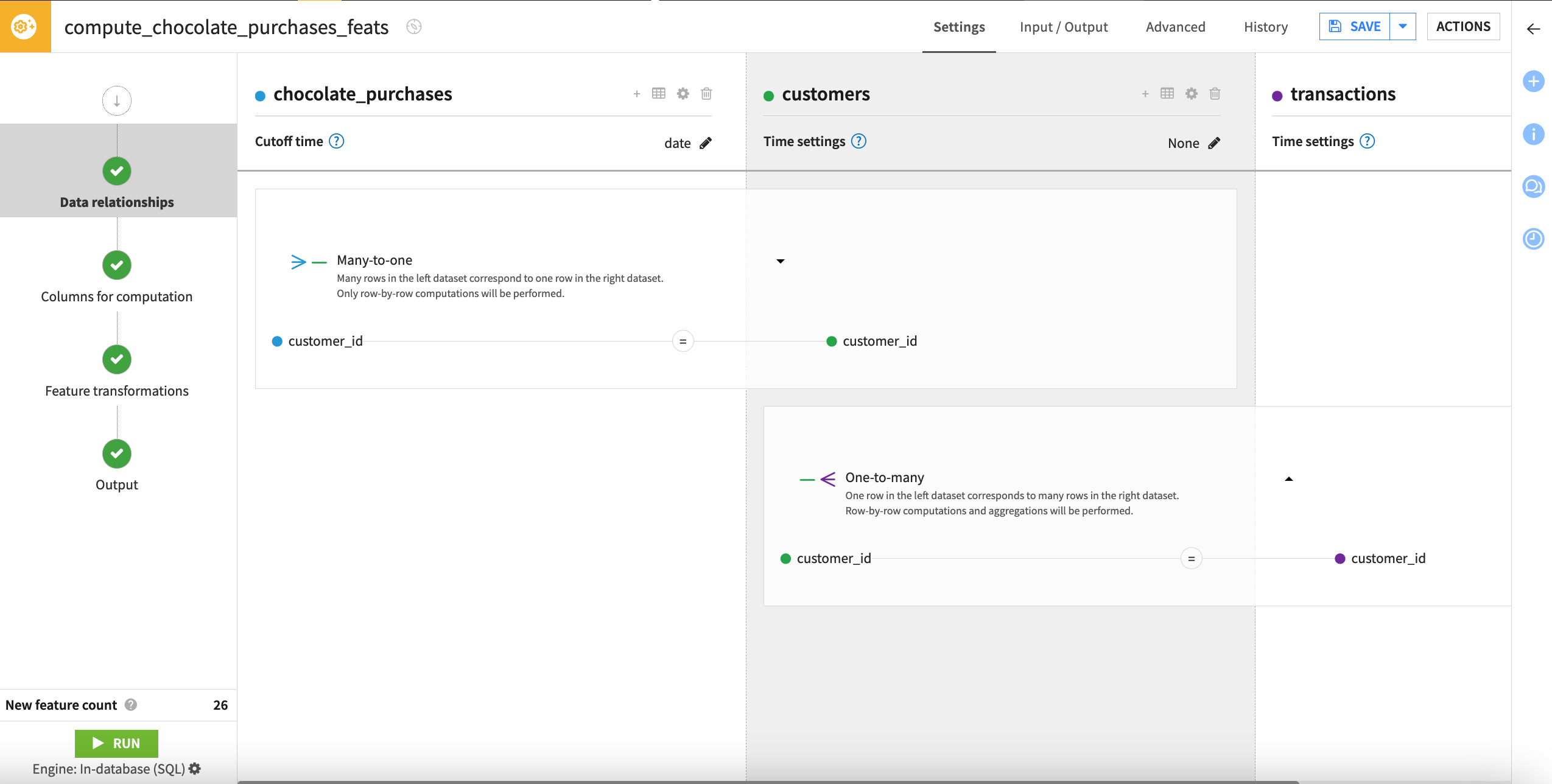
Next we’ll add the final enrichment dataset, transactions, which we’ll join in from the customers dataset. Customers has a one-to-many relationship with transactions, because each customer in the customers dataset can be listed multiple times in the transactions dataset, as each customer can have many transactions.
Next to the customers dataset name, click on the + icon to Add an enrichment dataset.
Select transactions as the Enrichment dataset.
Set the Time index to a Date column. The transaction_date column will be autoselected, as it’s the only date column. This column makes sense to use as a time index because we wouldn’t want to generate features based on future transactions.
Click Save, and return to the Data relationships step.
Check the join key, which has been automatically set to customer_id on each dataset. We can leave this as is. Since this relationship is one-to-many, the join key will be used as the group key when computing aggregations, so we will compute new features per customer.
Click on Select the relationship between join keys, and select One-to-many.
Note
You can also add a time window to enrichment datasets. Time windows are based on the time index column and allow you to further narrow the time range used in feature generation.
With our data relationships set, we can select the columns on which we want to run computations.
Choose columns for computation#
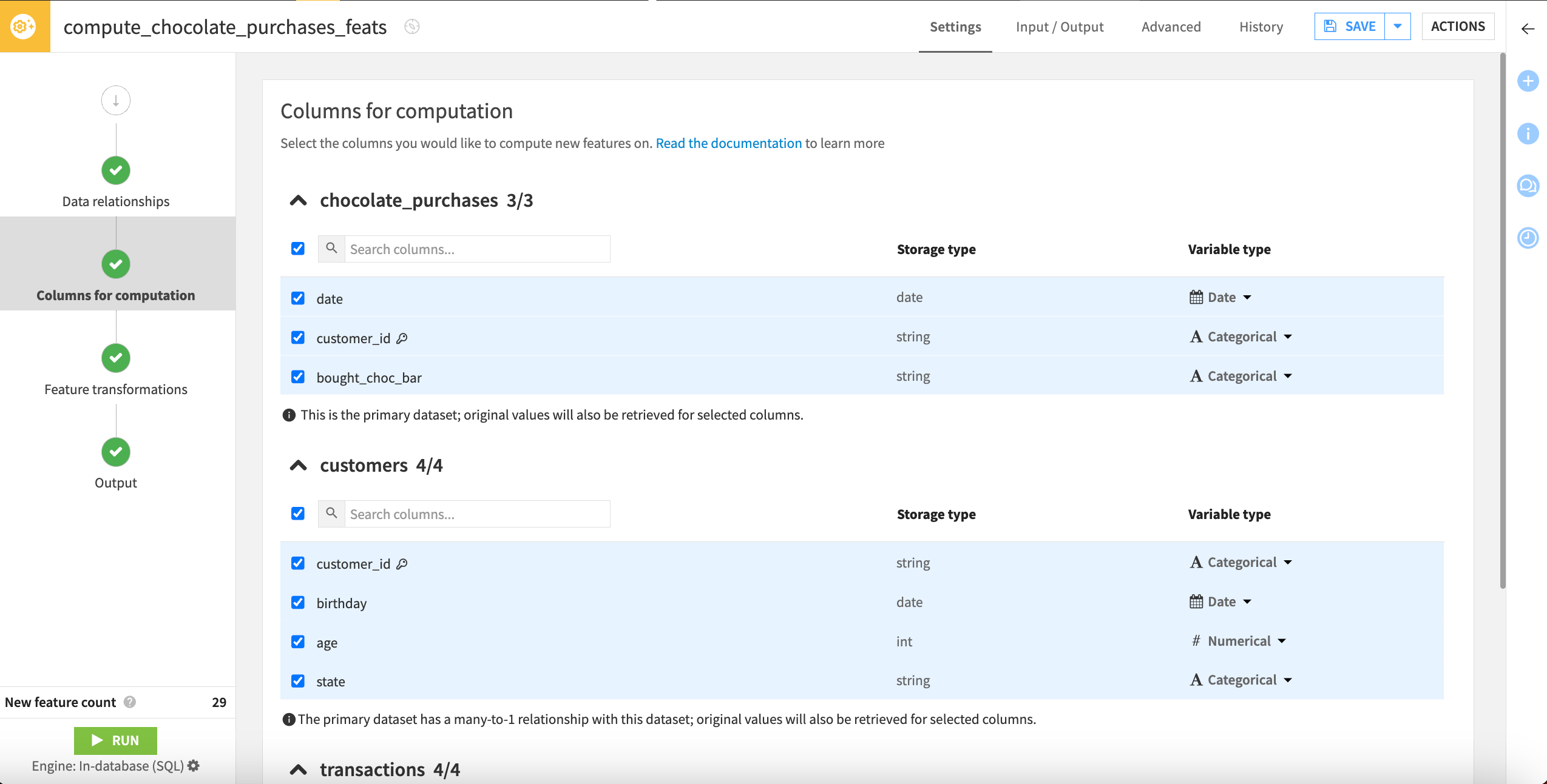
Navigate to the Columns for computation step. Here, you can select which features you want to run computations on and change variable types if needed. The variable type, along with the relationships we previously configured, affect the type of transformations that can be performed on selected columns.
For example, numerical columns can be aggregated by average, minimum, maximum, or sum, and date columns can be transformed at the row level into day of month, day of week, hour, week, month, or year.
Because this recipe can generate many features, it’s important to select only the columns you want to compute new features on. Let’s deselect some columns that don’t make sense to include.
Under the customers and transactions datasets, deselect the customer_id columns, which are the join keys (denoted with a key icon) and not useful to compute new features on.
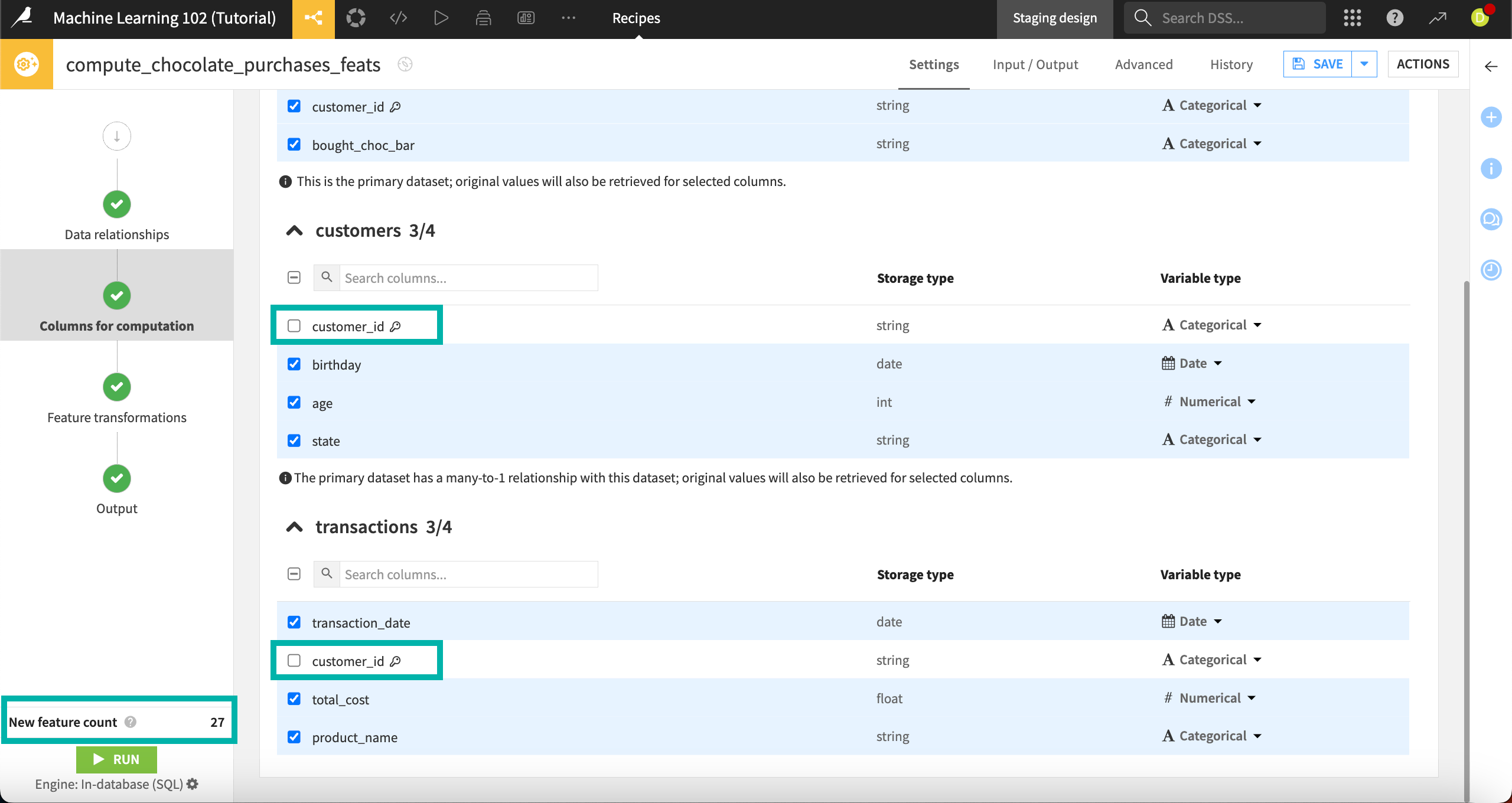
Note that when you change the column selection, the New feature count in the bottom left drops from 29 to 27. This lets us know how many new columns we’ll generate in the output dataset. It’s a good idea to keep an eye on this, particularly if your computations are taking a long time or consuming a lot of memory.
Check the Variable types on the right for each column. You can change these with the dropdown menus offering appropriate variable types based on the storage type. In our case, the types are appropriate and can be left untouched.
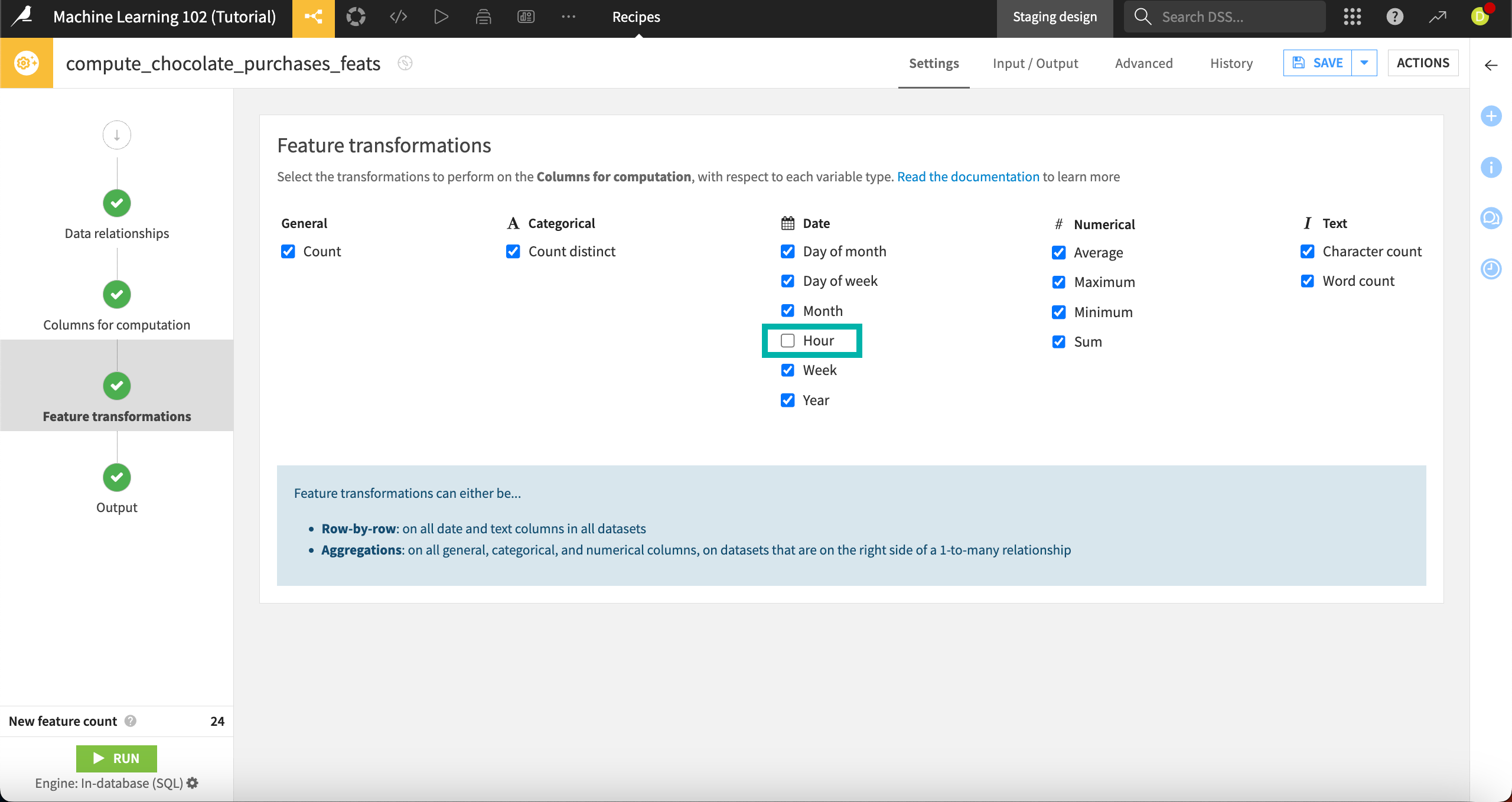
Select feature transformations#
Next, on the Feature transformations step, we can select the transformations we want to compute for each variable type.
Feature transformations can be performed on either:
A single row at a time, which occurs on all date and text columns in all datasets, or
Many rows at a time, which occurs on all general, categorical, and numerical columns, on datasets that are on the right side of a one-to-many relationship.
To reduce the number of new features generated, let’s deselect the hour transformation. Our dates don’t have this level of detail, so it doesn’t make sense to keep it.
Under Date, deselect Hour.
This drops the New feature count to 24.
Go to the Output step. This shows a preview of the output dataset’s schema, including all columns from the primary dataset and the 24 new features that the recipe will compute — 27 columns in total.
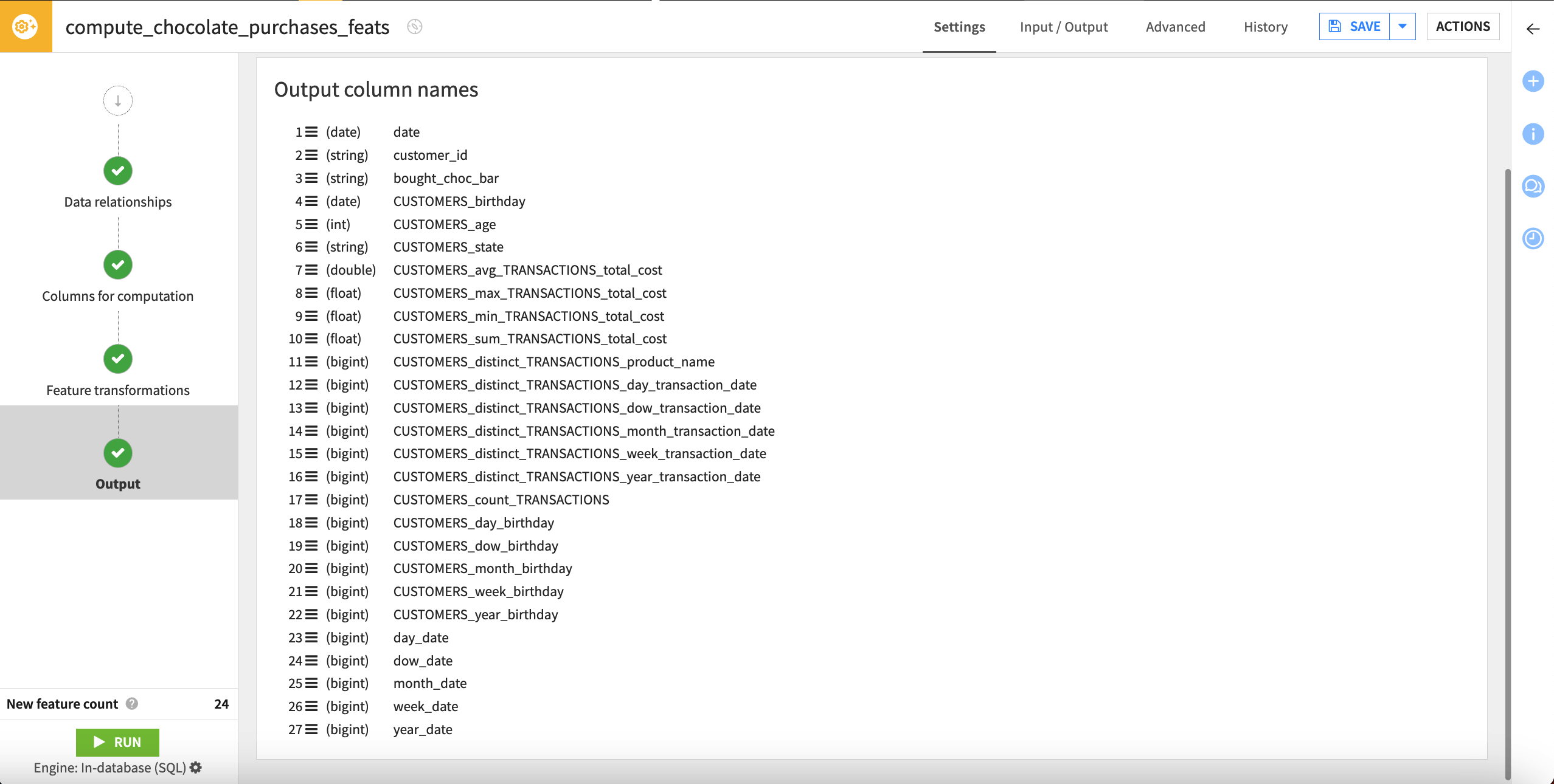
Each computed column name includes the original dataset, original column, and the transformation that took place.
In this step, you can also select View query to view the SQL query or Convert to SQL recipe if you want to modify it programmatically.
Explore and use output dataset#
After configuring the settings, we’re ready to run the recipe and view the resulting dataset.
Click Run to execute the recipe.
After the job finishes, select Explore dataset chocolate_purchases_feats.
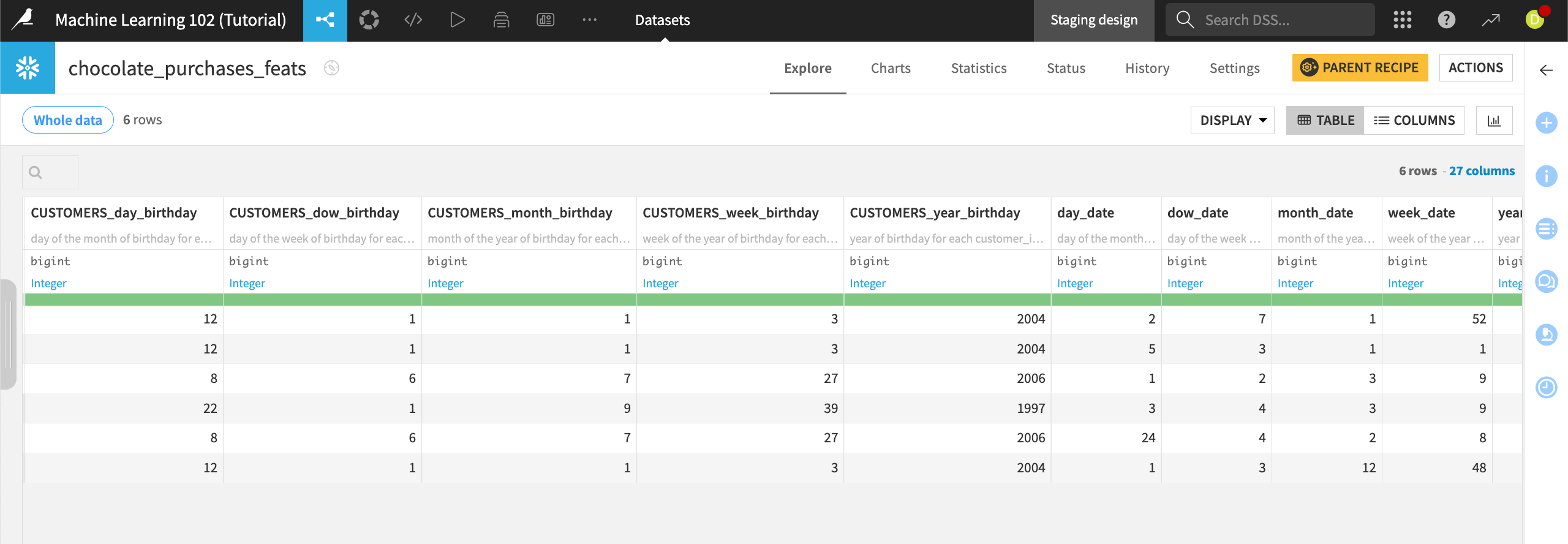
The dataset contains 27 columns, including the original three from the primary dataset and the 24 new computed features.
In addition to the column name, each column header contains a description of how the feature was computed.
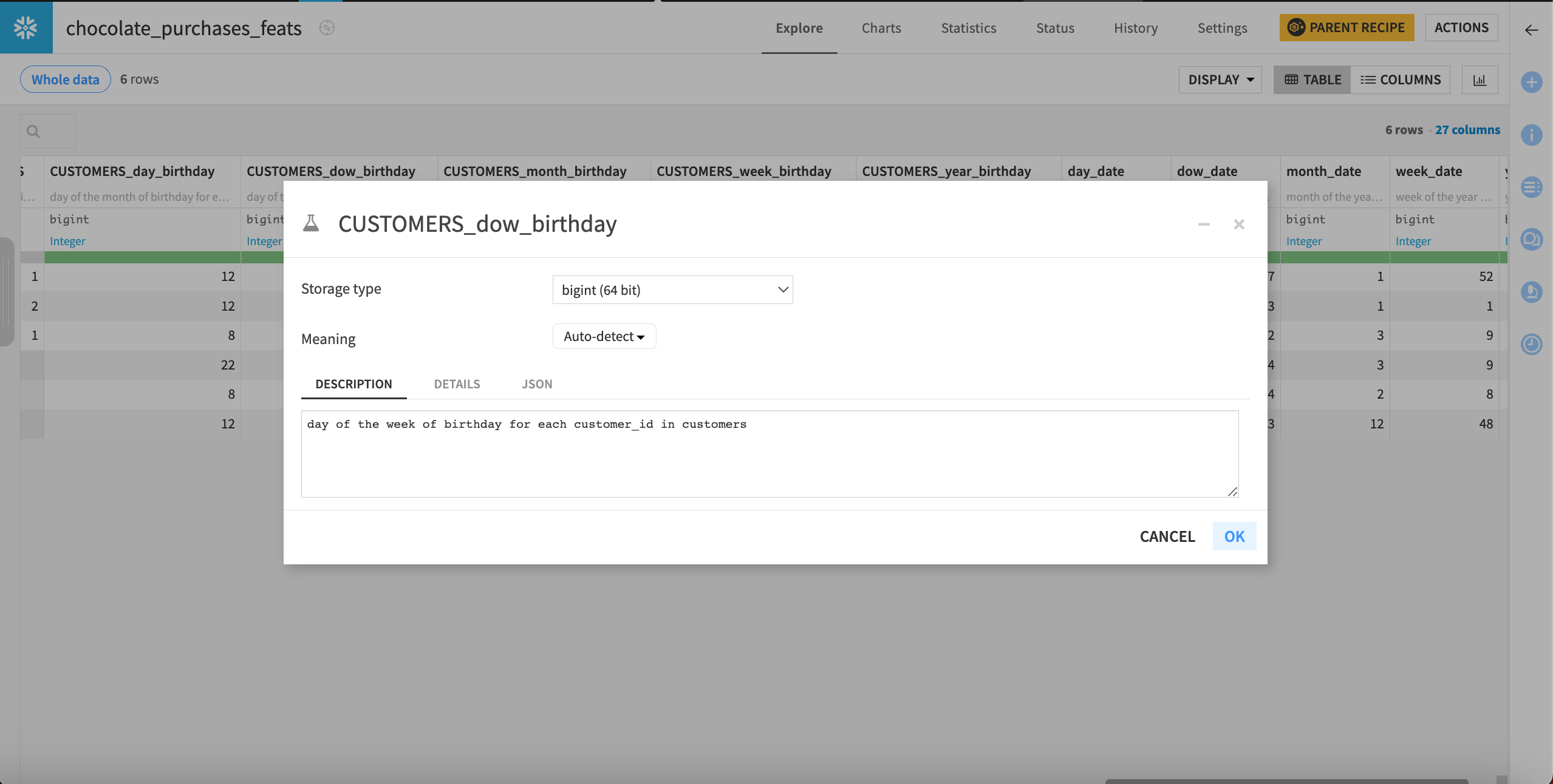
To view a full description, click on the column header dropdown and select Edit column schema.
For example, the column CUSTOMERS_dow_birthday gives the description “day of the week of birthday for each customer_id in customers.”
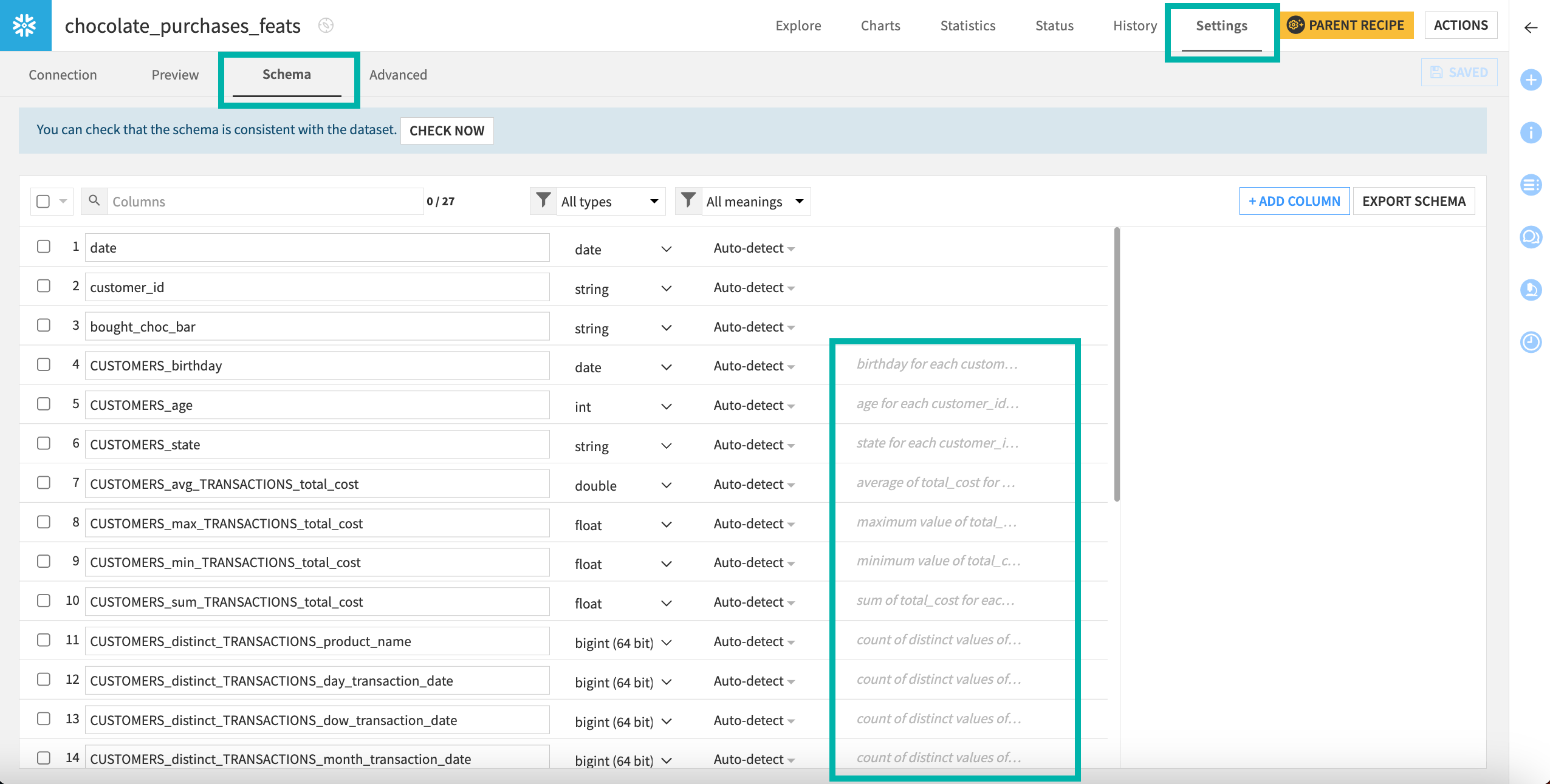
You may also visit Settings > Schema to explore descriptions for all columns.
This recipe has generated some interesting new features such as the month when chocolate bars were purchased (mo_date), and average transactions. Using these in a model, we could see if customers were more likely to buy chocolate depending on their age, month of purchase, or average cost of their transactions.
Next steps#
Congratulations! You’ve built a dataset with newly generated features, which is now ready for further use, either for deeper analysis or for a machine learning model. Note that you can perform feature reduction in the Lab after training a model to streamline its performance, especially if your Generate features recipe created many new features.