Concept | Model validation

Watch the video

Introduction

In the Concept | Predictive modeling lesson, we looked at a technique called supervised learning, where we use labeled training data to understand how different input variables can be used to predict an outcome. For example, a patient’ symptoms and family medical history can be used to predict whether a patient is sick or not sick.

Supervised learning models can learn from known historical information and then apply those known relationships to predict outcomes for individuals it hasn’t seen yet. How can we validate that a model will perform well on data it has not seen yet?

In this lesson, we’ll cover the techniques of using train and test sets, optimizing model hyperparameters, and controlling for overfitting — all crucial steps in the model validation process.

Train-test split

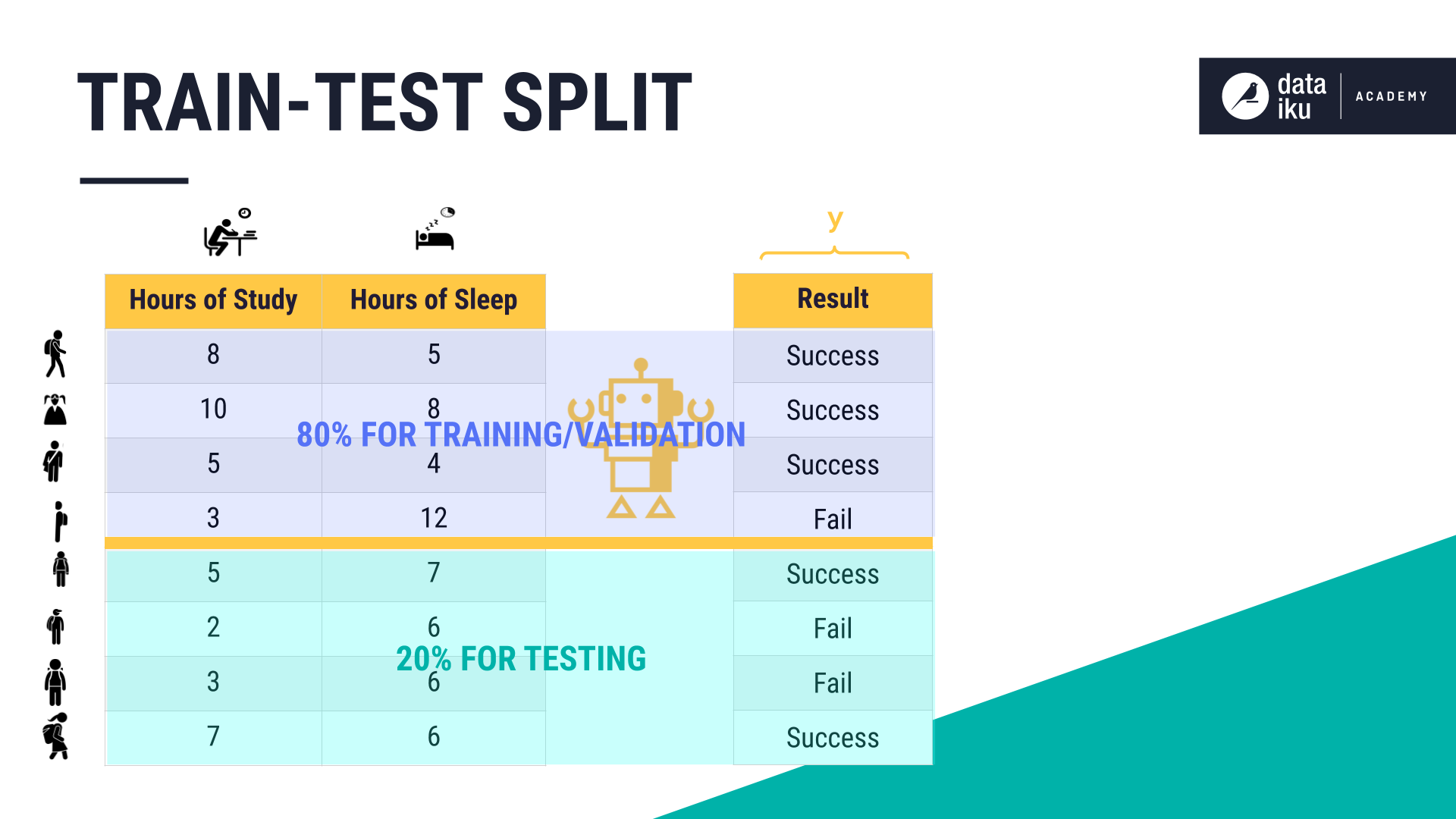
The first step in model validation is to split your known data, where we know the outcome, into a train and a test set.

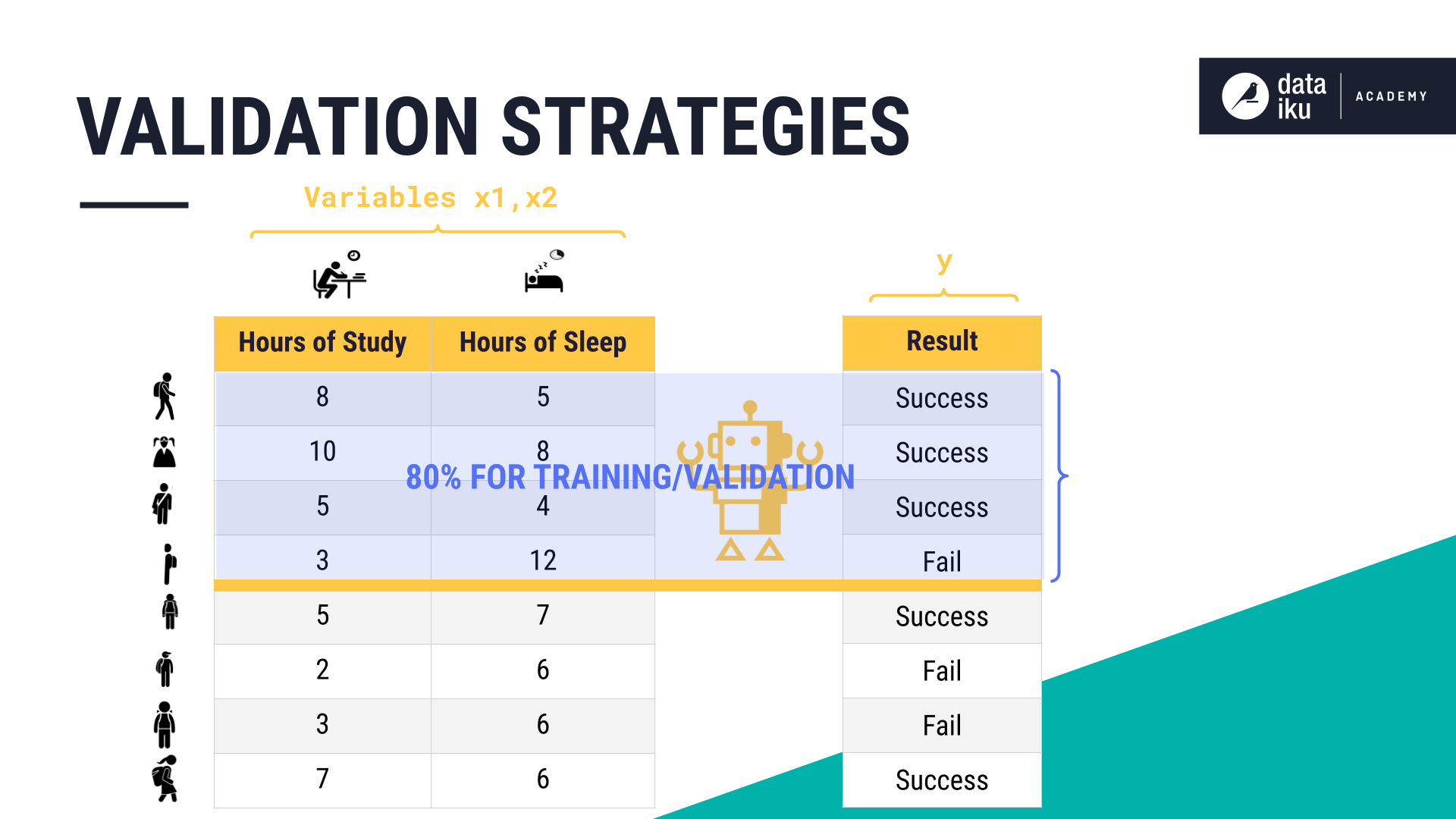
Here, we have a dataset of students. For each student, the dataset includes the number of hours they studied and hours they slept. These are the inputs to our model.

We will use our model to try to predict success or failure on a test.

Remember, this is known historical data. In supervised learning, we train a model based on data where we already know the outcome.

With this known dataset, we’ll take:

• 80% of rows as the train set.

• 20% of rows as the test set.

We’ll then train our model on the 80% set and evaluate its performance on the 20% test set, simulating how the model might perform on data it hasn’t seen before.

Parameters and hyperparameters

In machine learning, tuning the hyperparameters is an essential step in improving machine learning models. Let’s first make a quick distinction between the terms parameter and hyperparameter.

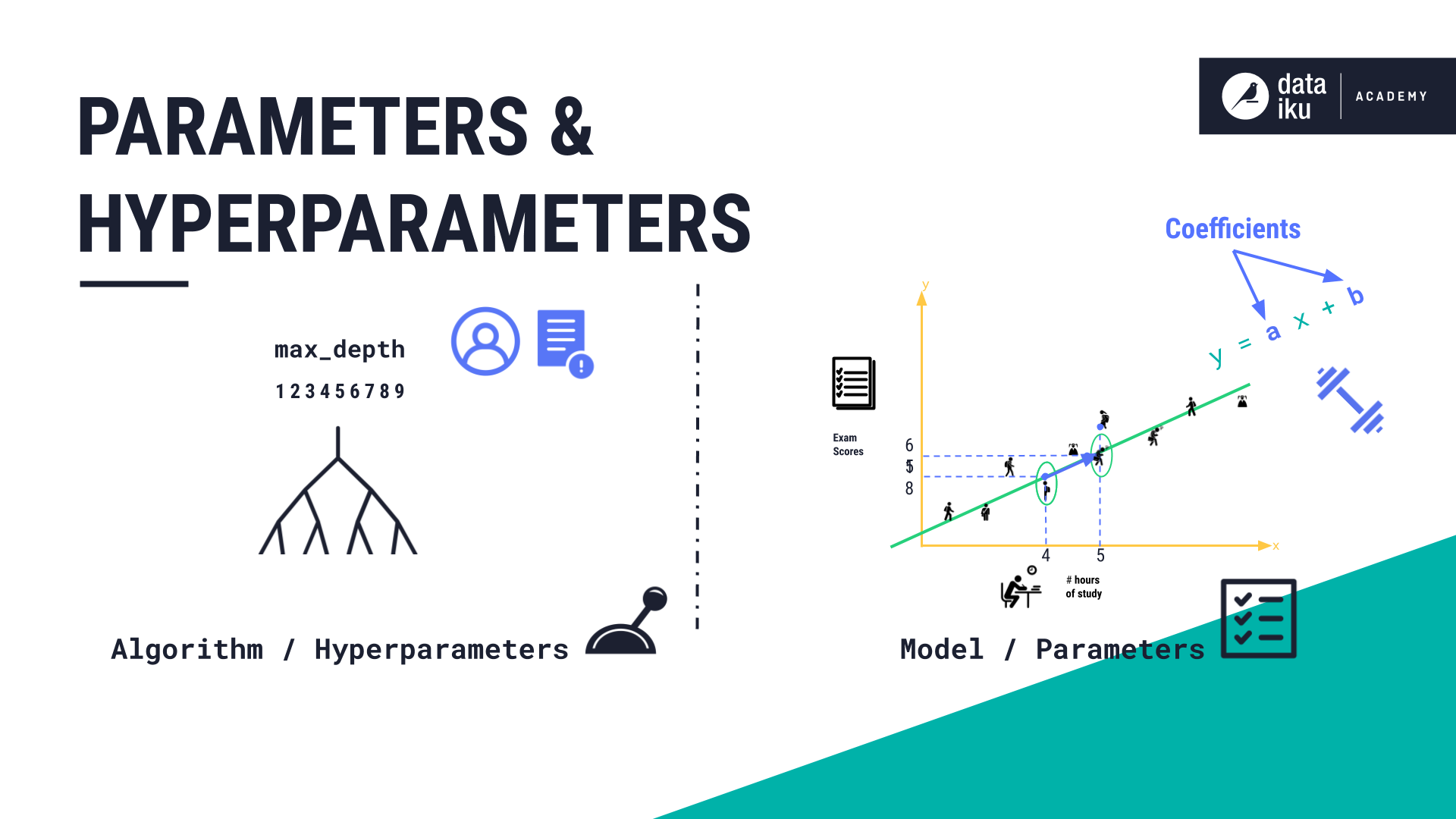
Model parameters are attributes about a model after it has been trained based on our known data. You can think of model parameters as a set of rules that define how a trained model makes predictions. These rules can be:

• an equation,

• a decision tree,

• many decision trees, or

• something more complex.

In the case of a linear regression model, the model parameters are the coefficients in our equations that the model “learns”–where each coefficient shows the impact of a change in an input variable on the outcome variable.

Algorithms’ hyperparameters are levers that can control how a model is trained by the algorithm. For example, when training a decision tree, one of these controls, or hyperparameters, is called max_depth. Changing this max_depth hyperparameter controls how deep the eventual model may go.

While it is an algorithm’s responsibility to find the optimal parameters for a model based on the training data, it is our responsibility, as ML practitioners, to choose the right hyperparameters which then control the algorithm.

Hyperparameter search

In machine learning, tuning the hyperparameters is part of the trial and error process, where our goal is to build the highest-performing model.

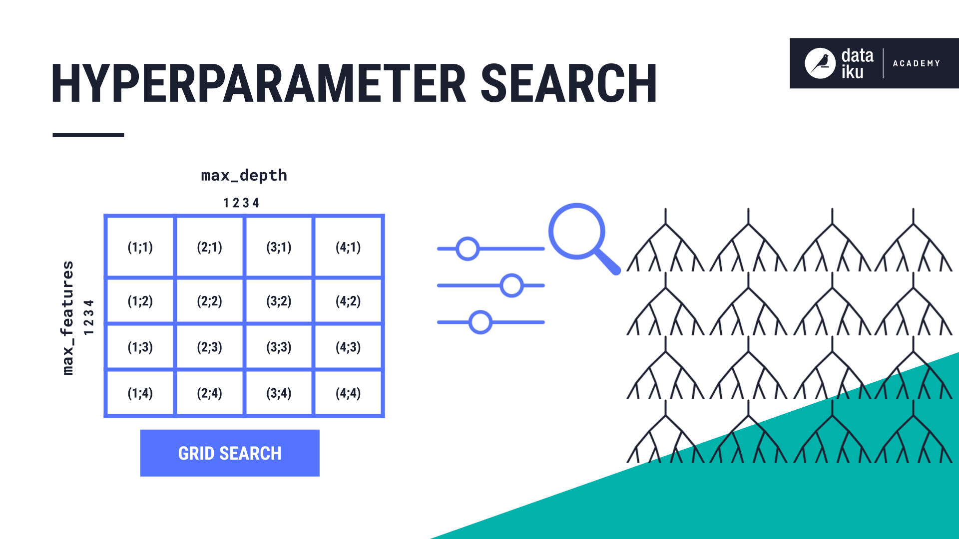
To find the best combination of hyperparameter values, machine learning practitioners perform a search. One classic method is called a grid search. An algorithm might have multiple hyperparameters that we need to find values for. A grid search will exhaustively test the values of all combinations of hyperparameters.

For example, if we wanted to train a random forest model, and try out the values 1, 2, 3 and 4 for the two hyperparameters max_features and max_depth, our grid would be 4 by 4, making 16 total combinations of our hyperparameter values. This means we will train 16 Random Forest models.

Next, we’ll discuss methods for validating this hyperparameter selection process. Now that we have 20% of the dataset set aside for testing, we can use the remaining 80% for the training and validation steps.

Validation strategies

The validation step is where we will optimize the hyperparameters for each algorithm we want to use. To perform this validation step, we’ll use the 80% of the dataset that we created during the train-test split step.

There are two common validation strategies: K-fold cross-validation and Hold-out set.

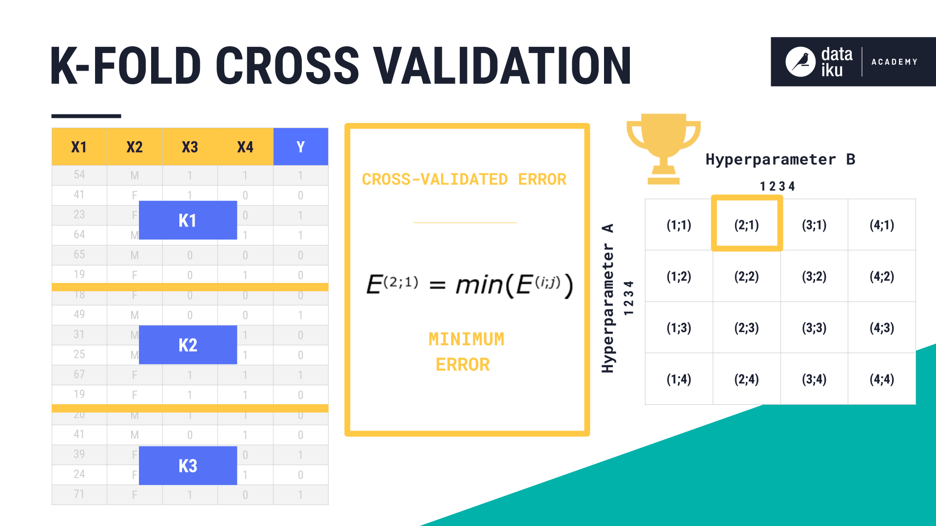
K-Fold cross-validation

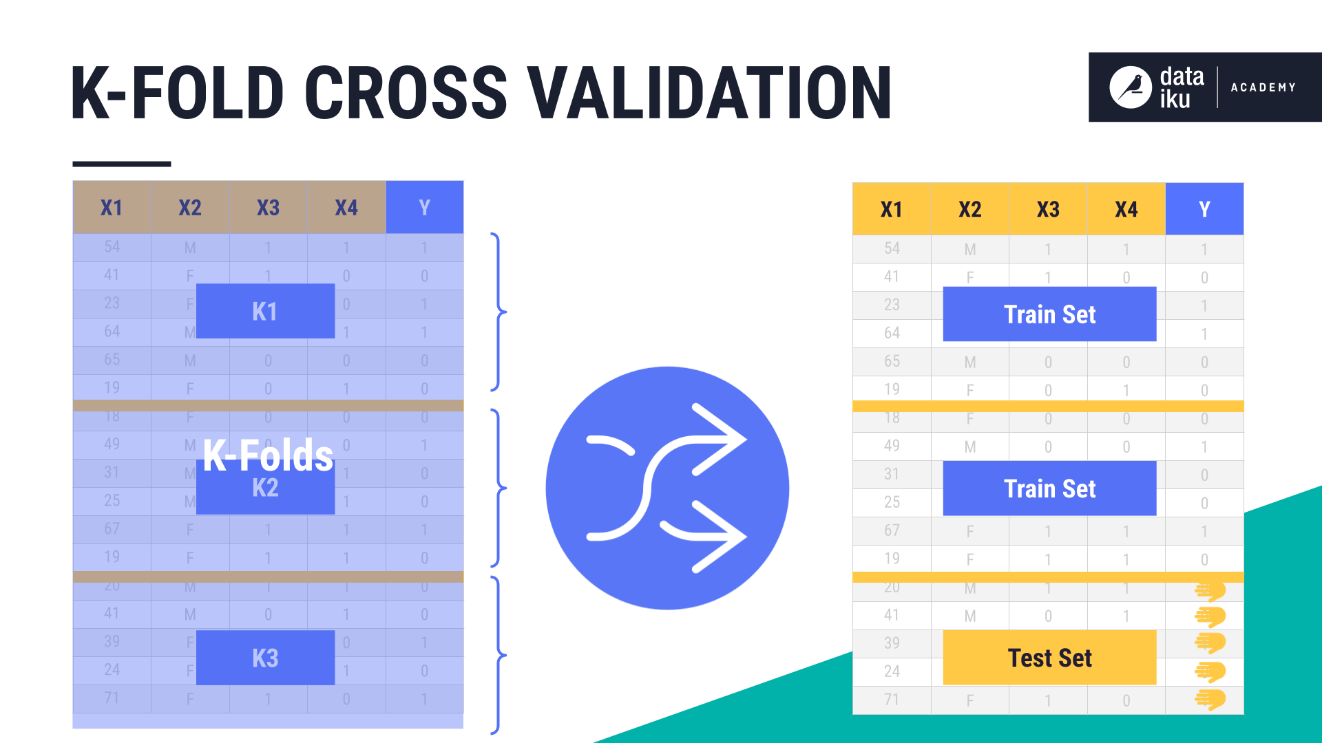
In K-fold cross-validation:

1. We take our training set, and split it into “K” sections or folds, where “K” represents some number, such as 3.

2. K-fold shuffles each fold, such that each fold gets the chance to be in both the training set and the validation set.

   

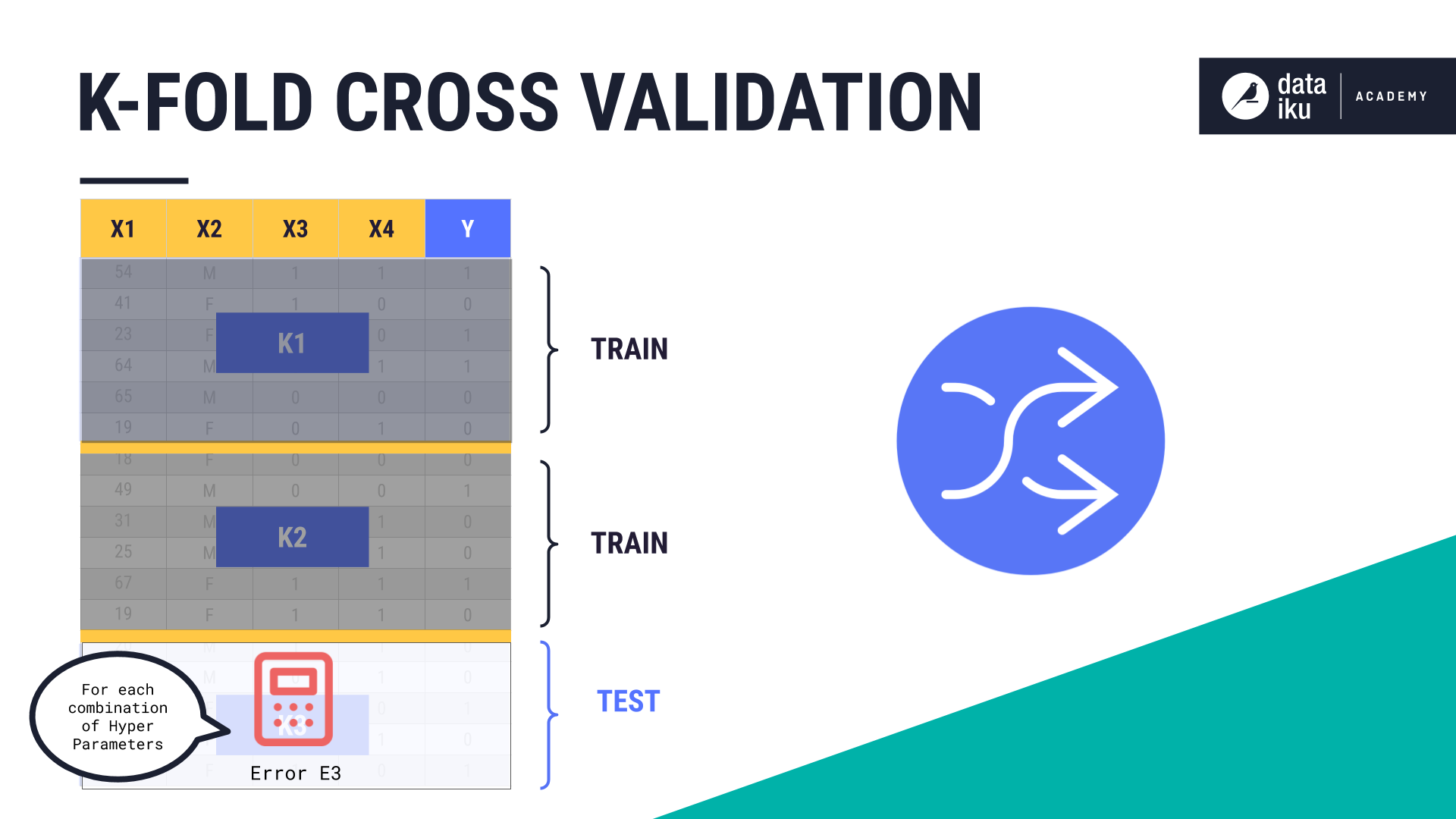
3. For each combination of hyperparameter values, we train the model on the folds assigned for training, and test and calculate the error on the folds assigned for validation.

4. The folds are then shuffled round-robin style, until the error has been calculated on all K-folds.

   

   The average of these errors is our cross-validated error for each combination of hyperparameters.

   

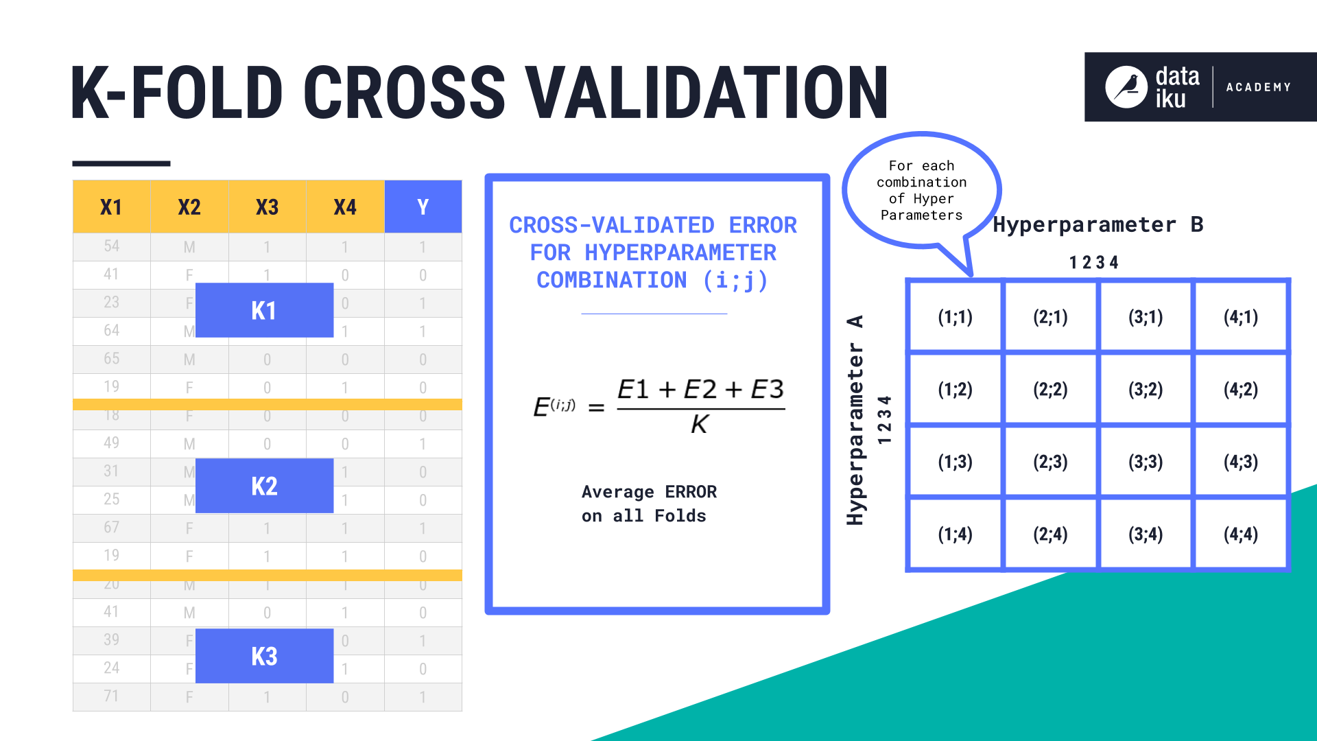
5. We then choose the combination of hyperparameters having the best cross-validated error, train our model on the full training set, and then compute the error on the test set–the one that we haven’t touched until now.

6. We can then use this test error to compare with other algorithms.

Hold-out validation

Another strategy is called Hold-out Validation. In this strategy, we simply set aside a section of our training set and use it as a validation set. For example, we could create a 60-20-20 split (train-validation-test). In this strategy, the sets are not shuffled.

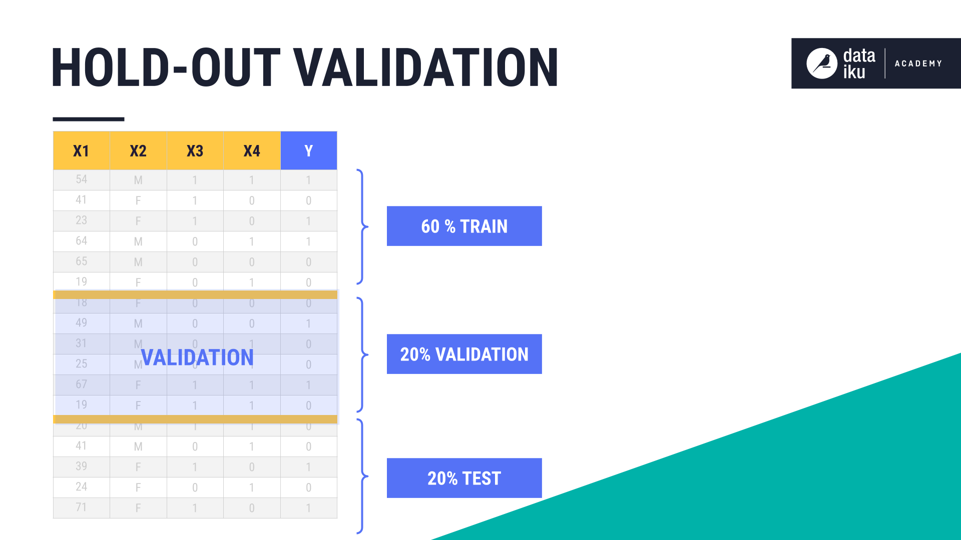
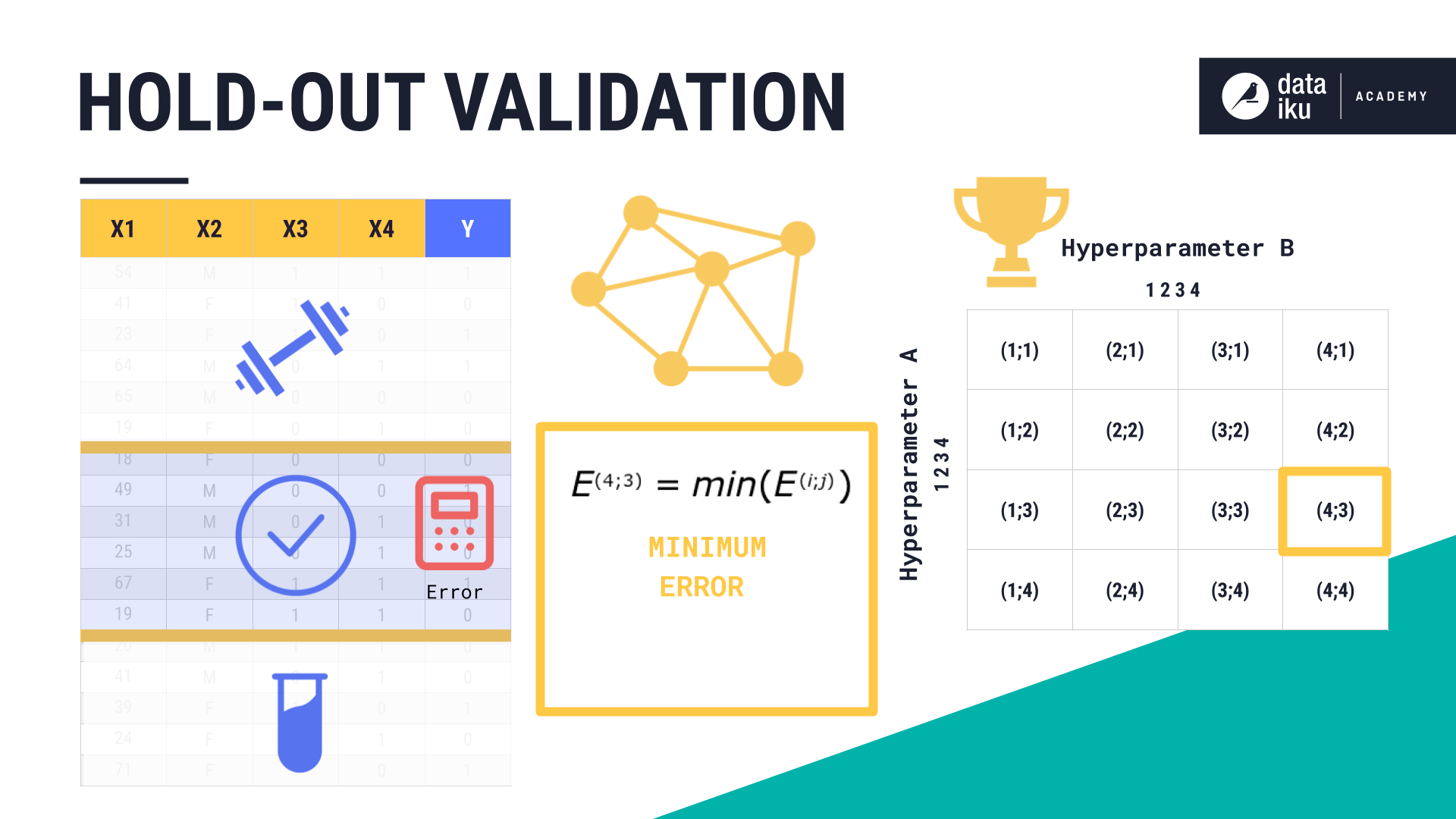
Instead, for each combination of hyperparameter values that we want to test, we would:

1. Calculate the error on our validation set.

2. Choose the model with the lowest error.

3. Calculate the test error on our test set.

This gives us a model that we can confidently apply to new, unseen data.

Validation strategy comparison

Let’s look at the pros and cons of each strategy we just learned about.

Validation type	Pros	Cons
K-fold	It is robust as it uses the entire training set, which results in less variance in the observations.	It takes up more time and computational resources.
Hold-out	It is less time consuming and consumes fewer computational resources.	It is not as robust.

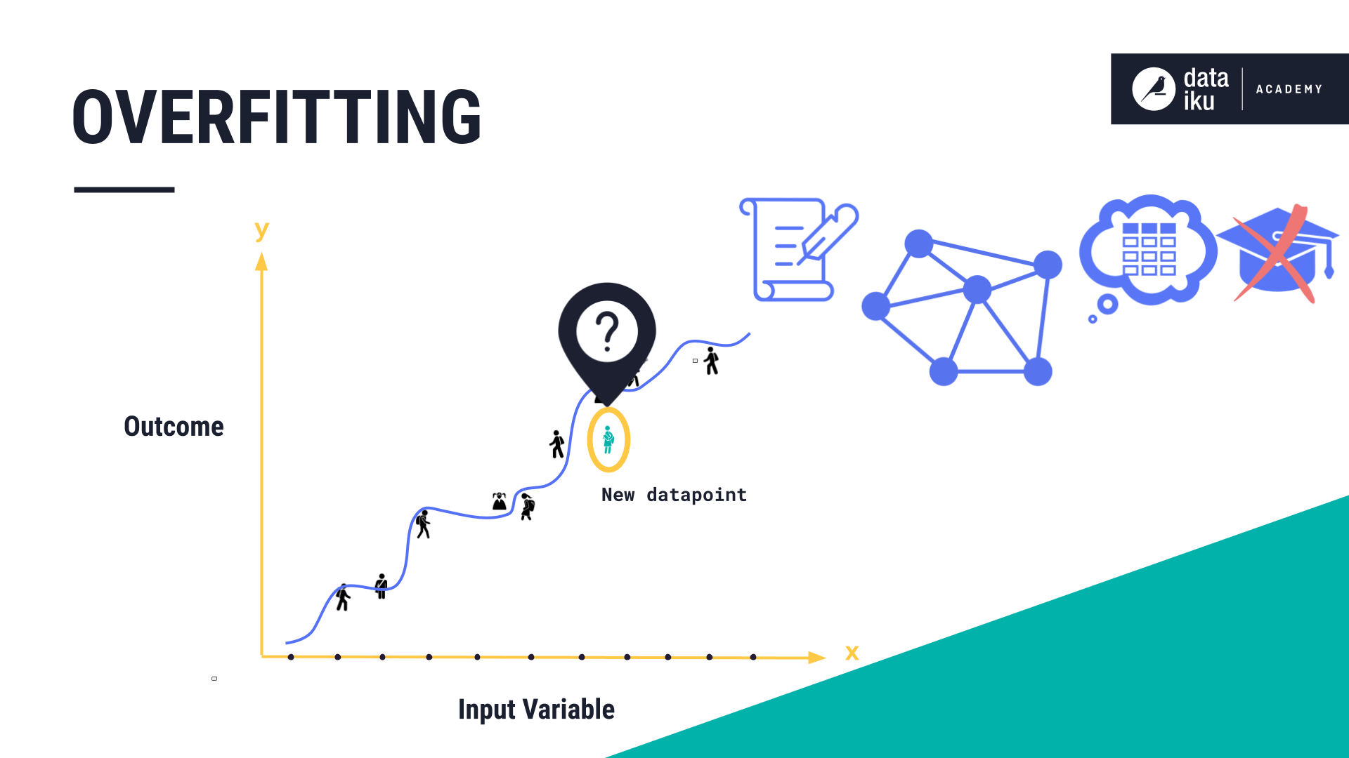
Overfitting

As we train our models and optimize hyperparameters to minimize some error calculation or other performance metric, we should take care to avoid the problem of overfitting.

Recall that we train machine learning models on known historical data. We ultimately want our models to be generalizable, meaning they should make good predictions on new (unseen) data.

Overfitting occurs when a model fits the historical training dataset too well. It means the model has simply memorized the dataset rather than learning the relationship between the inputs and outputs. It has picked up on the “noise” in the dataset, rather than the “signal” of true, underlying variable relationships.

As a result, the overfit model cannot apply what it has learned to new data and is unable to make a prediction.

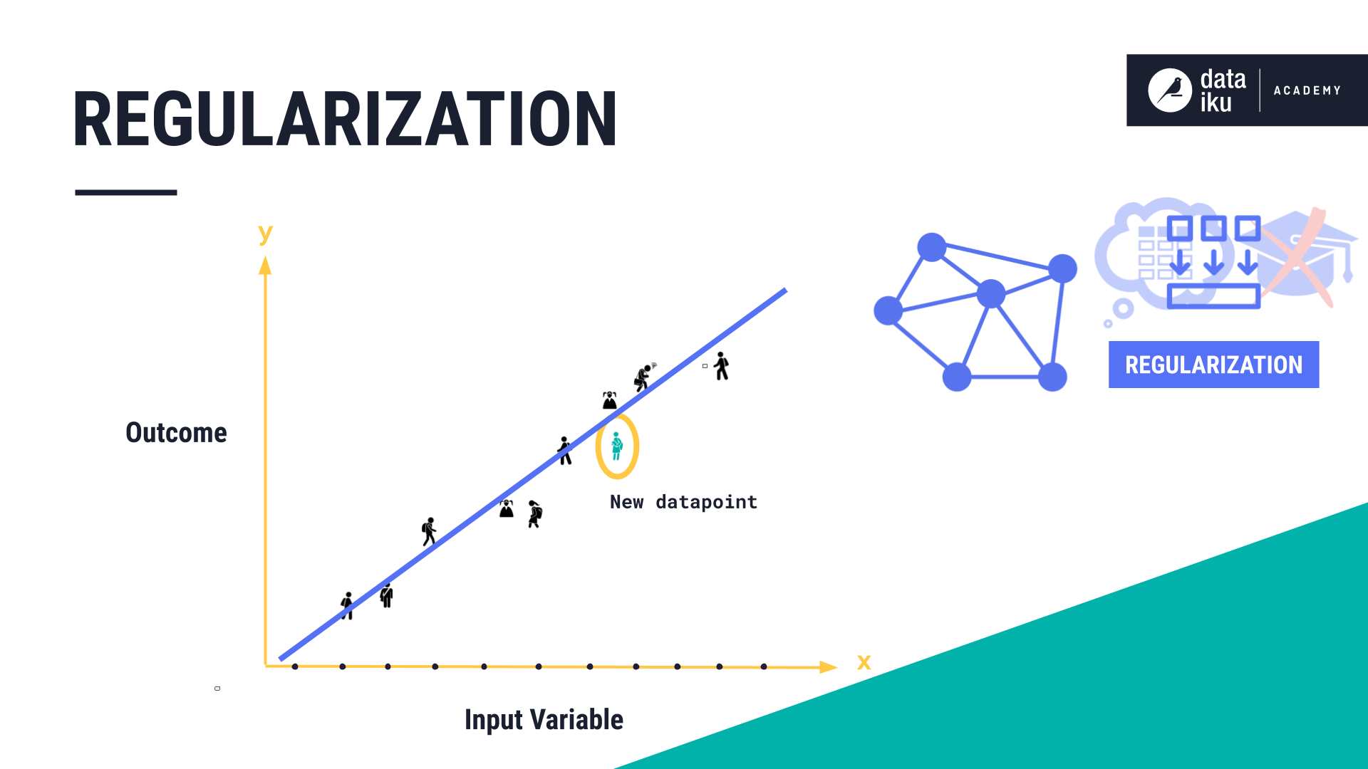
The remedy for overfitting is called regularization. Regularization is a technique to minimize the complexity of the model. The more complex the model - the more prone it is to overfitting. There are different methods for incorporating regularization into your model - most are specific to the algorithm you are using.

What’s next?

Now that you’ve completed this lesson about model validation, you can move on to discussions about algorithms including classification and regression, and model evaluation techniques.