
Concept | Model evaluation#
Watch the video
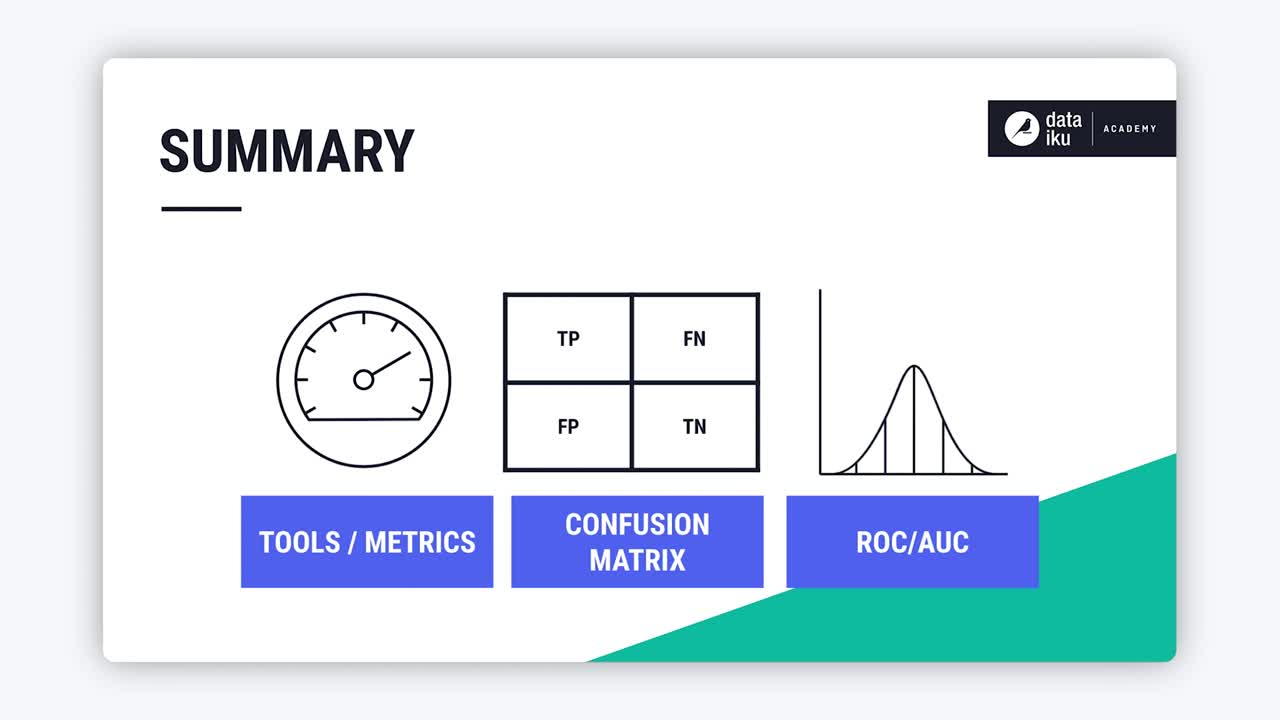
There are several metrics for evaluating machine learning models, depending on whether you are working with a regression model or a classification model. In this lesson, we’ll mainly focus on tools for evaluating classification models including a confusion matrix and ROC/AUC.
Confusion matrix#
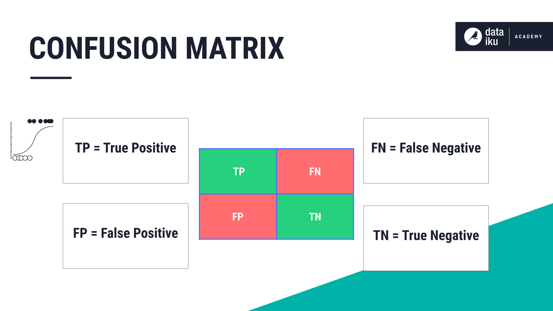
One tool used to evaluate and compare models is a confusion matrix. A confusion matrix is used to evaluate a classification model.
In our binary classification example, our classes are Succeed and Fail. When we feed data with known outcomes into the model, we’ll know if the model made correct predictions or not.
Once we have the model’s predictions, we can assign one of four labels to each prediction.
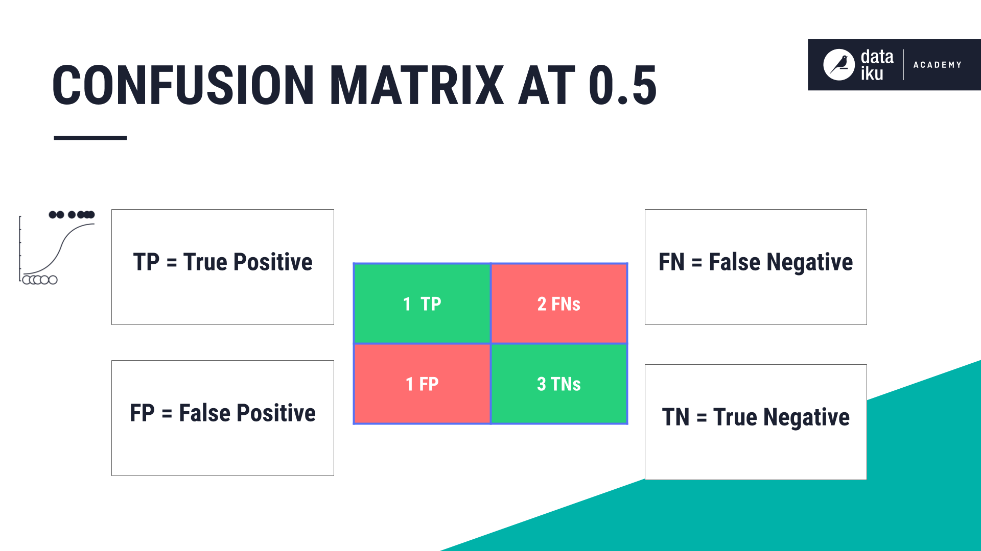
The correct predictions are labeled as TP or TN, where:
TP, or a true positive, is the count of Trues or Succeeds that the model correctly predicted.
TN, or true negative, is the count of Falses or Fails that the model correctly predicted.
The incorrect predictions will be labeled as FP or FN (see the Type I and Type II Errors section below for further information).
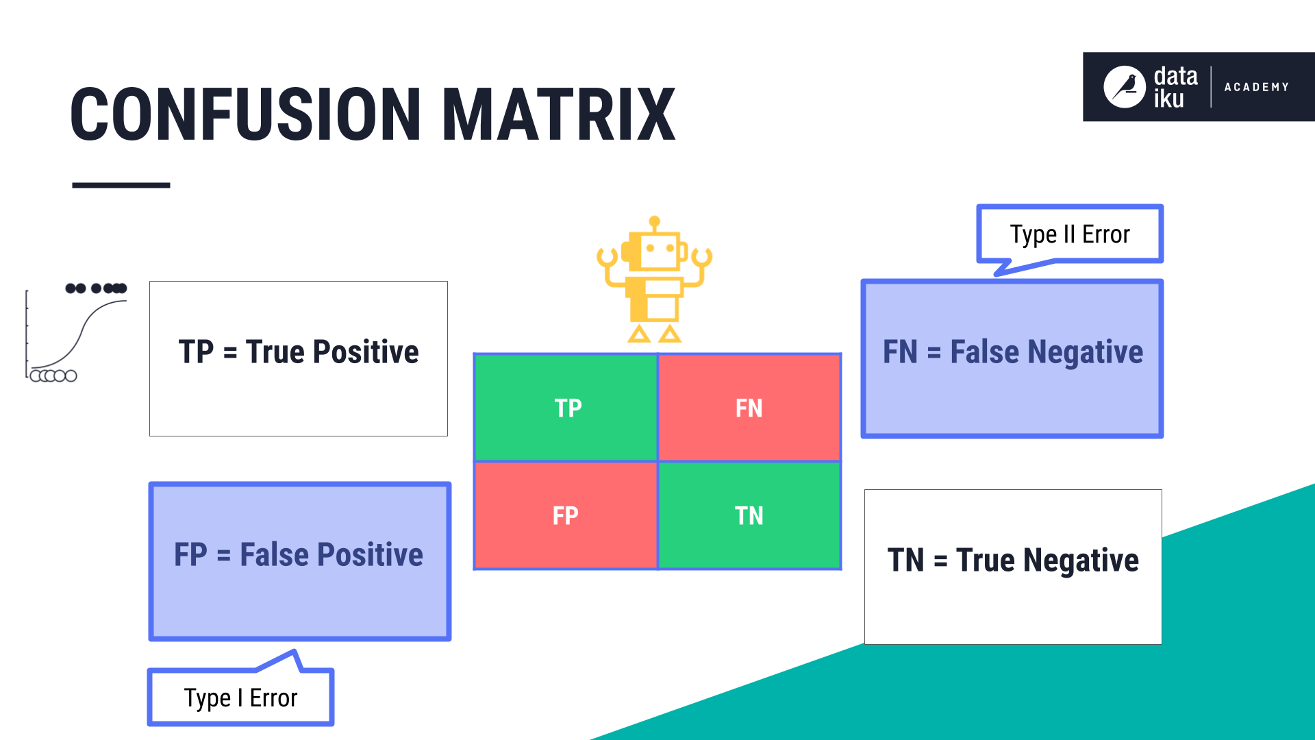
Type I and type II errors#
An FP, or false positive, is known as a Type I Error. It’s the count of Falses or Fails that the model predicted incorrectly. In other words, this is where the model predicted Succeed where it should have predicted Fail.
An FN, or false negative, refers to a case in which the model predicts False, when the result is actually True. In this case, the model would have predicted Fail when it should have predicted Succeed. This is known as a Type II error.
This is important because in prediction there will always be errors. Depending on our use case, we have to decide if we’re more willing to accept higher numbers of Type I or Type II errors.
For example, if we were classifying observations as either having cancer or not having cancer, we would be more concerned with a high number of false negatives. In other words, we would want to minimize the number of predictions where the model falsely predicts that a model’s test result doesn’t indicate cancer.
Similarly, if we were classifying a person as either guilty of a crime, or not guilty of a crime, we would be more concerned with high numbers of false positives. We would want to reduce the number of predictions where the model falsely predicts that a person is guilty.
Building a confusion matrix#
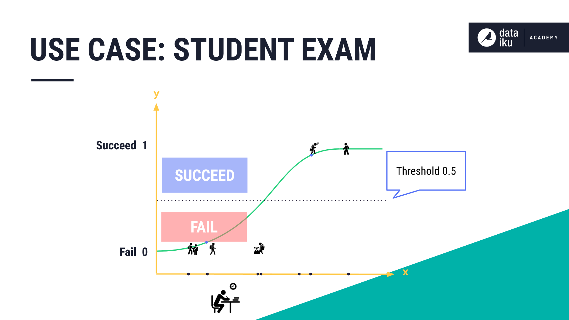
Let’s build a confusion matrix using our Student Exam Outcome use case where:
The input variable, or feature, is the hours of study.
The outcome we’re trying to predict is Succeed or Fail.
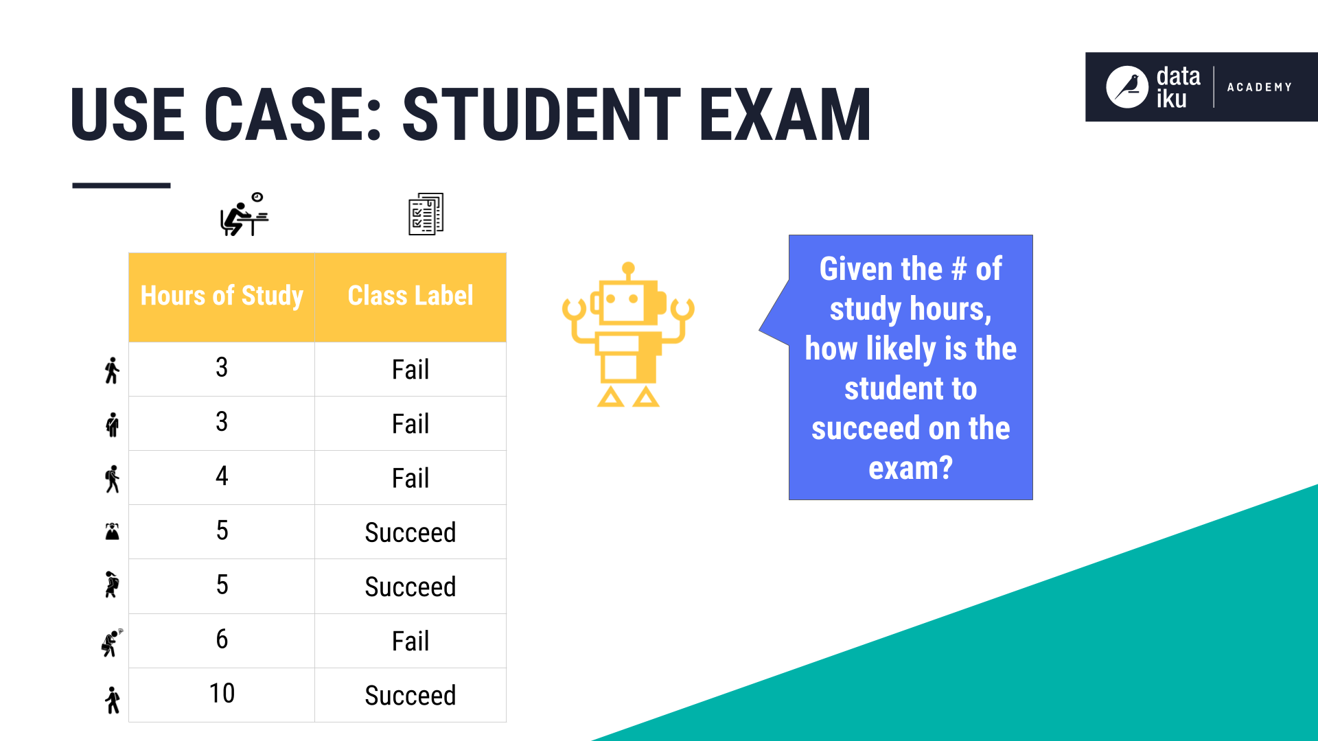
In this example, we’ve trained the model using a logistic regression algorithm. We’ve used a probability threshold, or cutoff point, of 0.5, which is about halfway between Succeed and Fail.
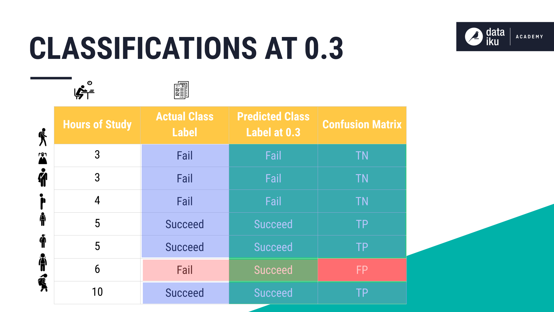
To create our confusion matrix, we’ll need to refer to our results that show the actual class label, along with the predicted class label.
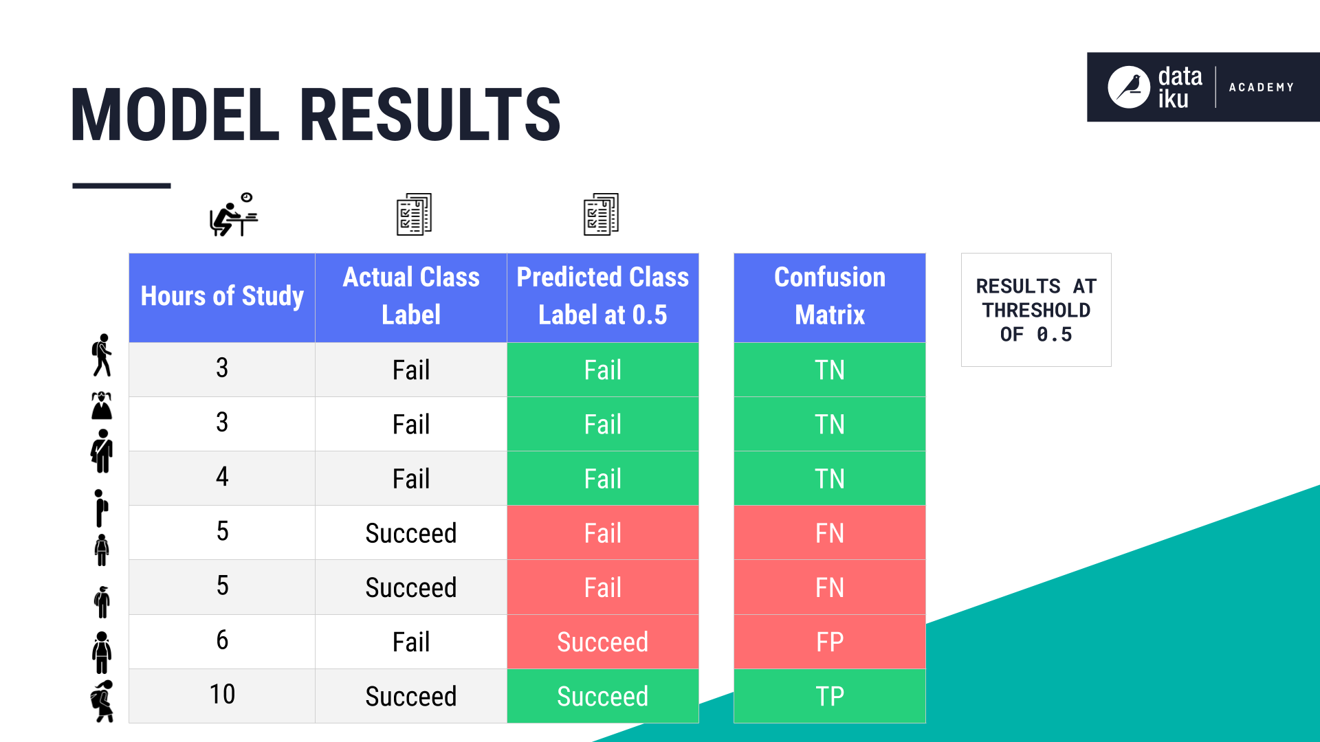
A confusion matrix is a simple table format. Since we only have two possible outcomes, our table has only two columns and two rows.
Testing a different threshold#
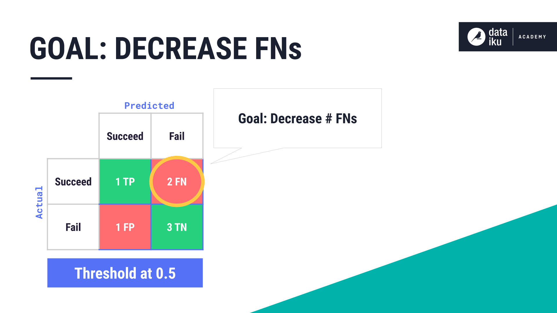
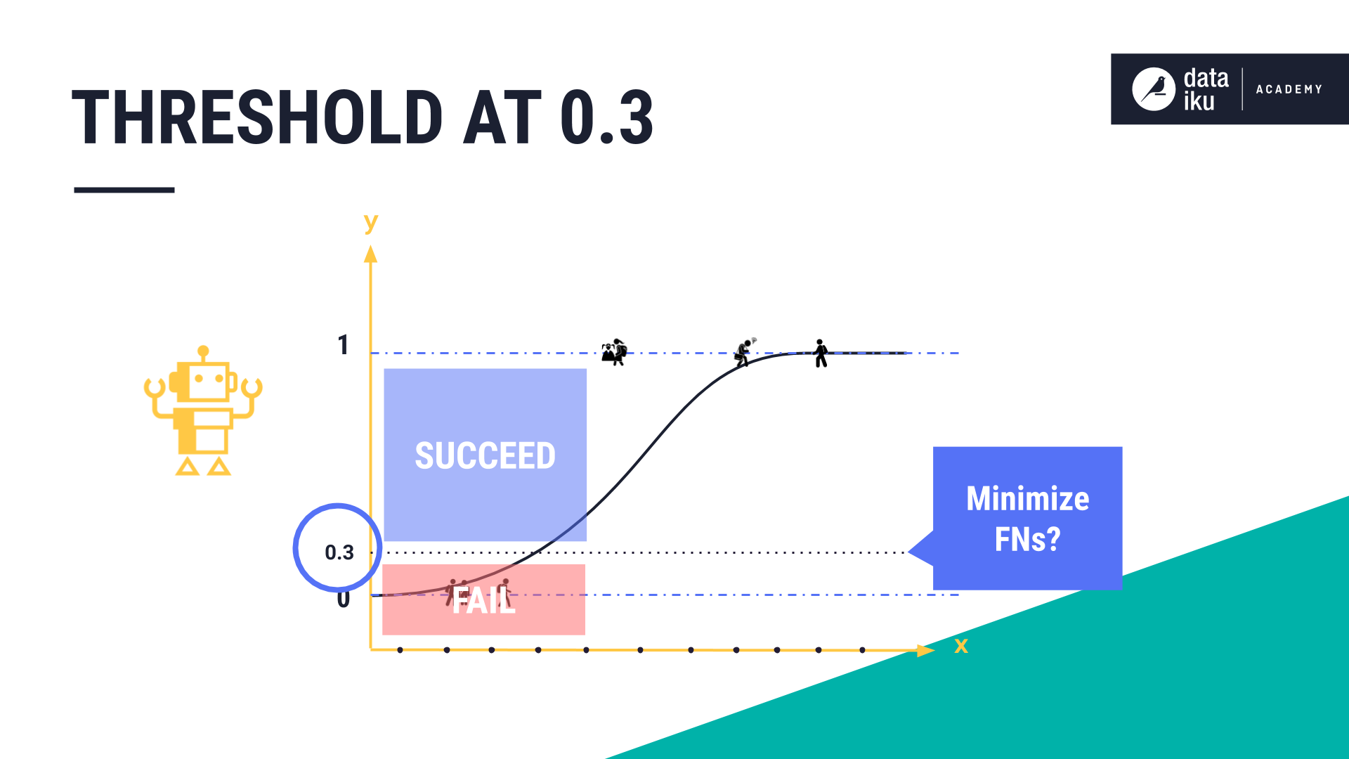
Let’s say our goal is to minimize the number of false negatives, or the number of Fail predictions that have an actual outcome of Succeed. That is, we’ve decided that we’re more willing to accept too many false positives (predicting that a student who actually Failed would Succeed) than too many false negatives.
To minimize the number of false negatives, we can try a different threshold.
Note
The threshold is the cutoff point between what gets classified as Succeed and what gets classified as Fail.
For our exam outcome use case, we’ll attempt to decrease the number of false negatives by trying out a different threshold, this time 0.3, and applying the model again.
Once again, at a threshold of 0.3, the model has made some correct and some incorrect predictions.
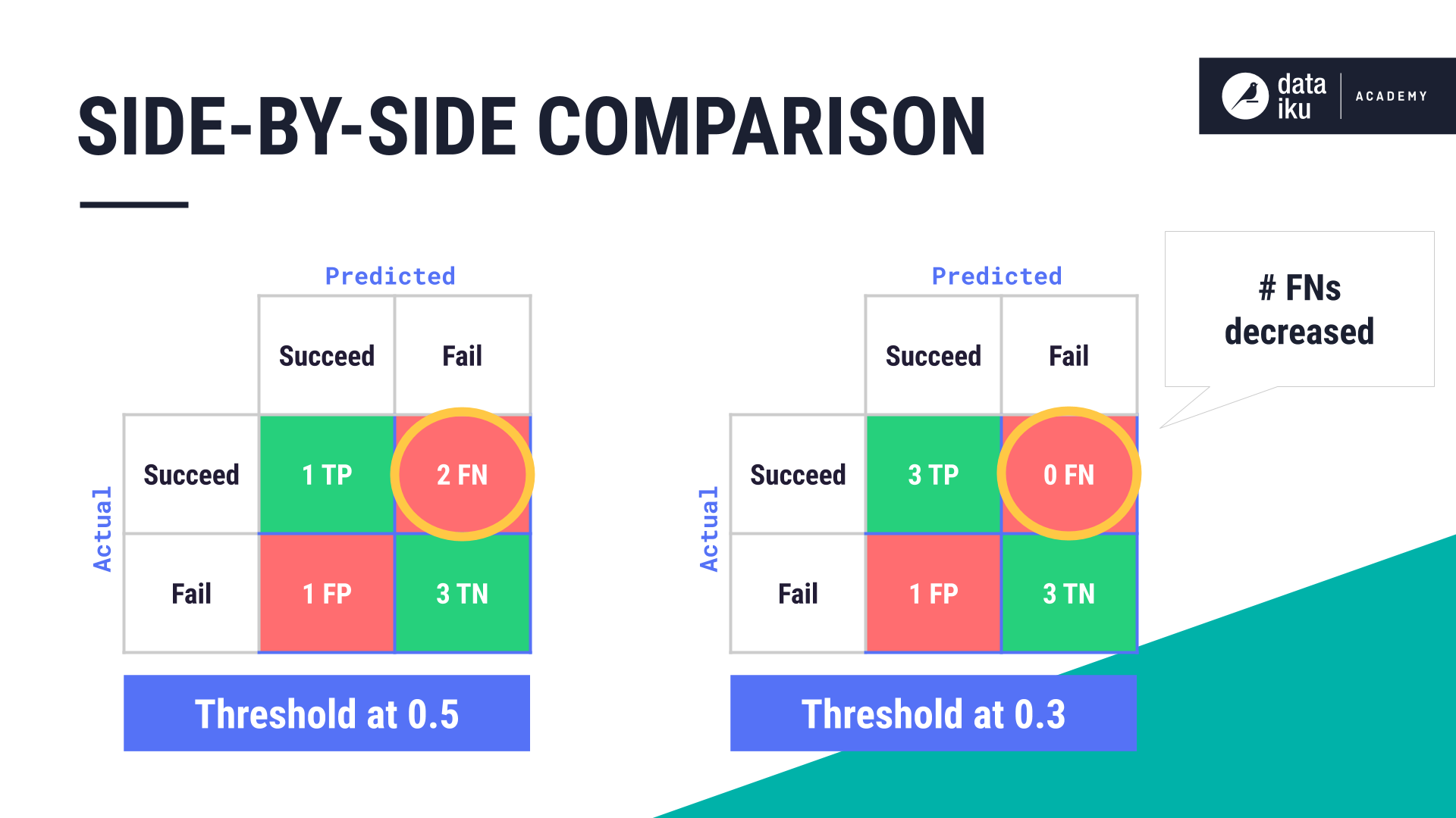
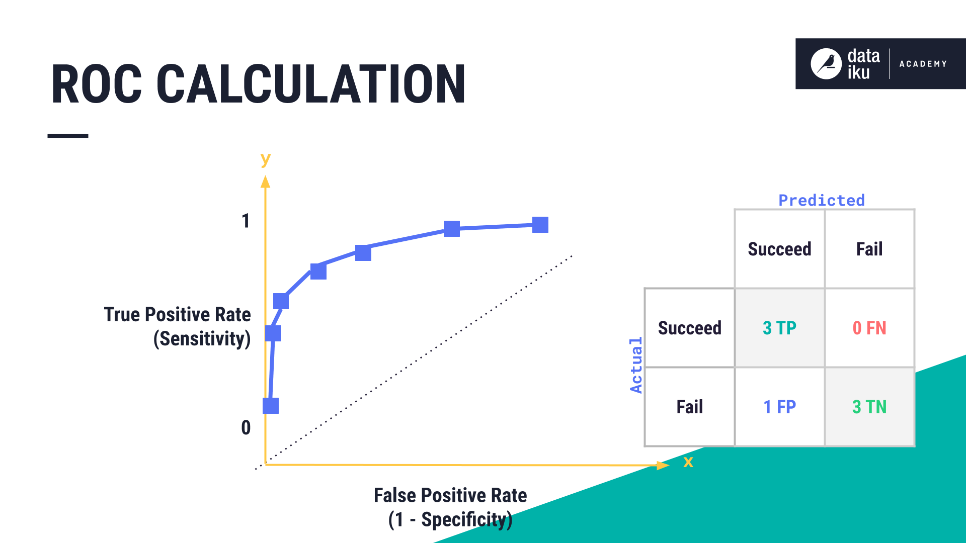
Adding these results to our confusion matrix, we get:
3 cases that are actually negative, or Fail, that the model predicted to be negative. These are the true negatives or TNs.
3 cases that are actually positive, or Succeed, that the model predicted to be positive. These are the true positives or TPs.
1 case that’s actually negative that the model predicted to be positive. This is the false positive or FP.
0 cases that are actually positive that the model predicted to be negatives. These are the false negatives or FNs.
Compared to the threshold of 0.5, the number of false negatives has decreased.
In our use case, using logistic regression, the more optimal threshold seems to be 0.3 with the observations that we’ve tested so far.
As you can see, creating a confusion matrix for every possible threshold would be too much information to compare. Thankfully, there are metrics to speed up the process.
Metrics to evaluate classification models#
Common metrics used to evaluate classification models are based on:
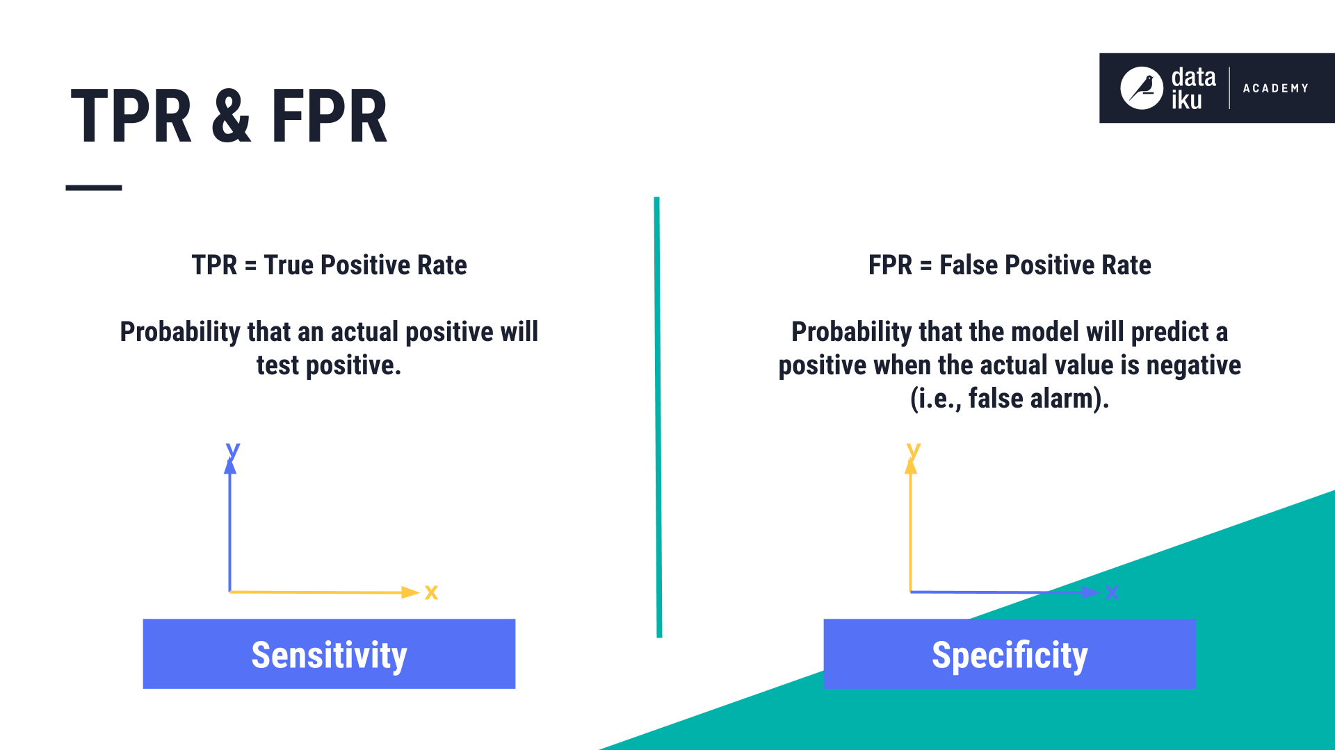
The TPR, i.e. true positive rate, that tells us what proportion of Succeed samples were correctly classified and is shown on the Y axis. It’s also known as sensitivity.
The FPR, i.e. false positive rate, that tells us what proportion of Fail observations were incorrectly classified as Succeed and is shown on the X axis. It’s also known as specificity.
ROC curve#
Using the TPR and FPR, we can create a graph known as an ROC curve, or receiver operator characteristic curve.
The True Positive Rate is found by taking the number of true positives and dividing it by the number of true positives plus the number of false negatives.
The False Positive Rate is found by taking the number of false positives and dividing it by the number of false positives plus the number of true negatives.
In plotting the TPR and FPR at each threshold, we create our ROC curve.
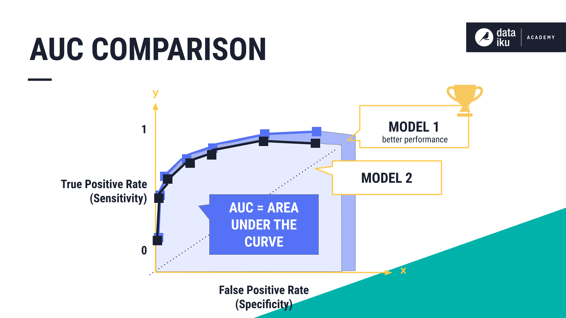
AUC score#
To convert our ROC curve into a single numerical metric, we can look at the area under the curve, known as the AUC. ROC curve and AUC scores are often used together. The ROC/AUC represents a common way to measure model performance.
We can compare models side-by-side by comparing their ROC-AUC graphs.
The AUC is always between 0 and 1. The closer to 1, the higher the performance of the model.
If one model has more area under its curve, and thus, a higher AUC score, it generally means that this model is performing better.
Other key metrics#
Other metrics used to evaluate classification models include Accuracy, Precision, and Recall.
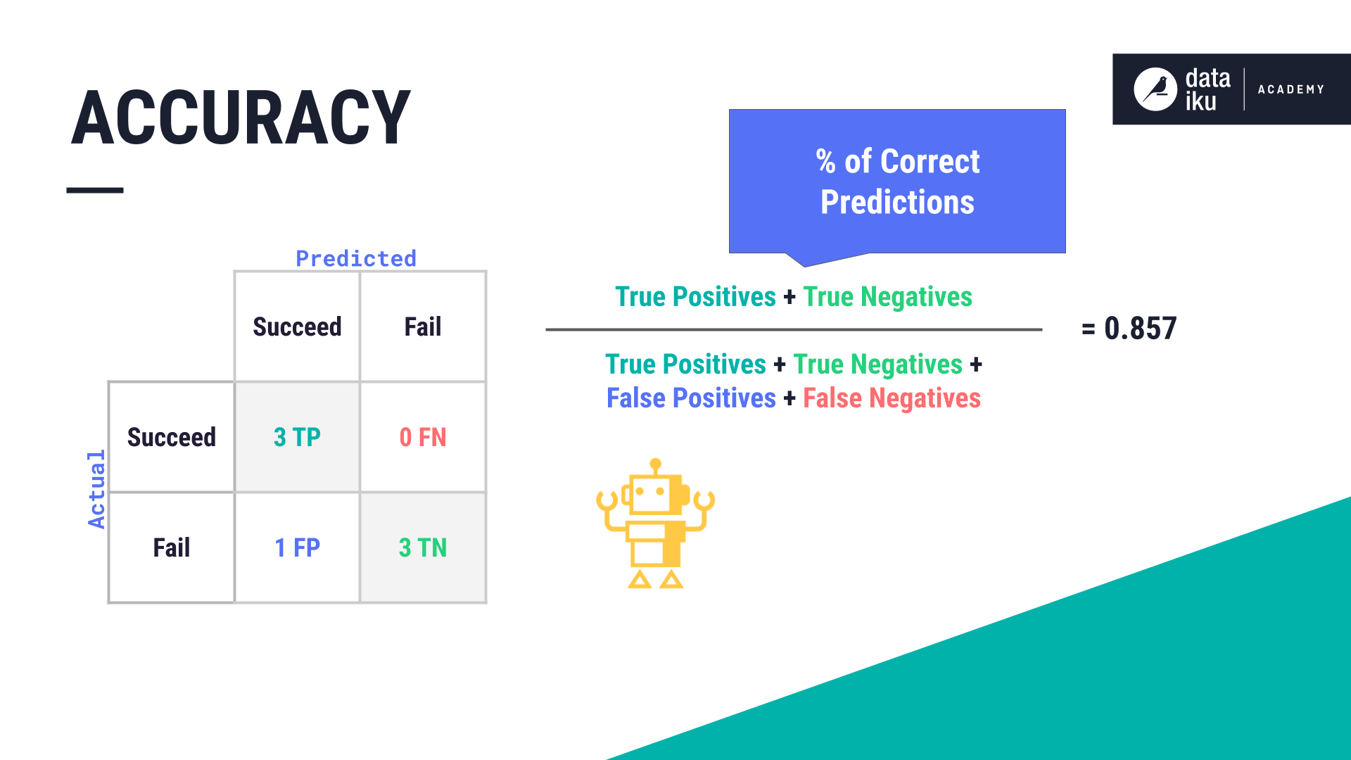
Accuracy#
Accuracy is a simple metric for evaluating classification models. It’s the percentage of observations that were correctly predicted by the model. We calculate accuracy by adding up the number of true positives and true negatives then dividing that by the total population, or all counts. The result is 0.857 in our case.
Caution
Accuracy seems simple but should be used with caution when the classes to predict aren’t balanced. For example, if 90% of our test observations were Succeed, we could always predict Succeed (and we would have a 90% accuracy score), however, we would never correctly classify a Fail.
Precision#
Precision is the proportion of positive results that were correctly classified (in our use case, these are the correctly classified Succeed results).
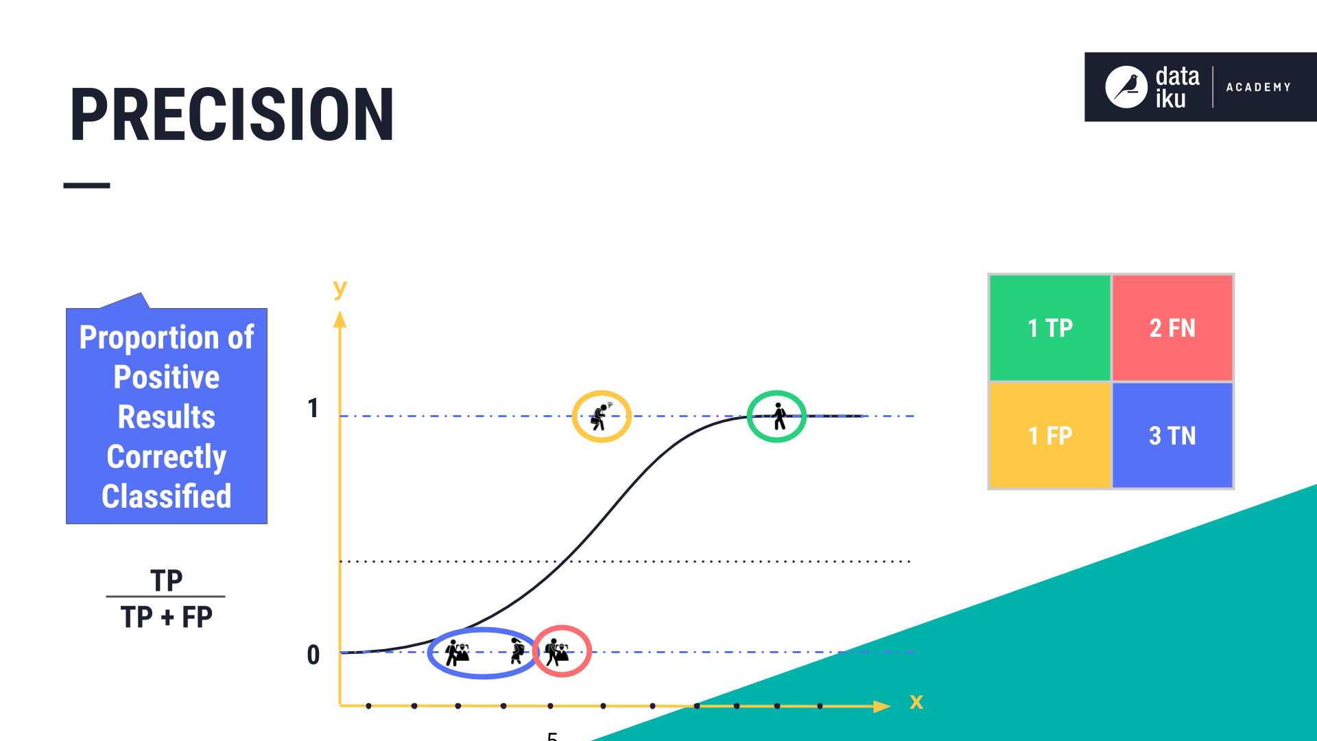
Precision can be compared to FPR, that, in our case, tells us what proportion of Fail observations were incorrectly classified as Succeed.
If we had many more test observations that were Fail (or Not succeed), resulting in an imbalance of the test observations, then we might want to use Precision rather than the FPR. This is because Precision ignores the number of True Negatives, i.e. the true Fails, so if there is an imbalance in our sample set then Precision isn’t affected.
Machine learning practitioners often use Precision along with another metric, Recall.
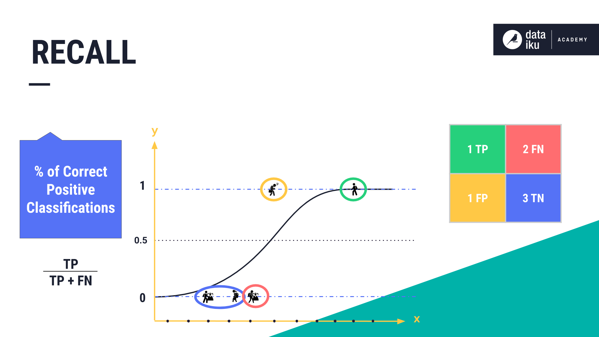
Recall#
Recall is the percentage of correct positive classifications (True Positives) from cases that are actually positive. In our case, this is the percentage of correct Succeed classifications.
Depending on our use case, we might want to check our number of False Negatives. For example, in our use case, if the model results in many false Fails, it might indicate that we failed to classify student observations correctly.
Metrics to evaluate regression models#
Now, let’s look at a few key metrics used to evaluate regression models: Mean Squared Error and R2 (or R-Squared).
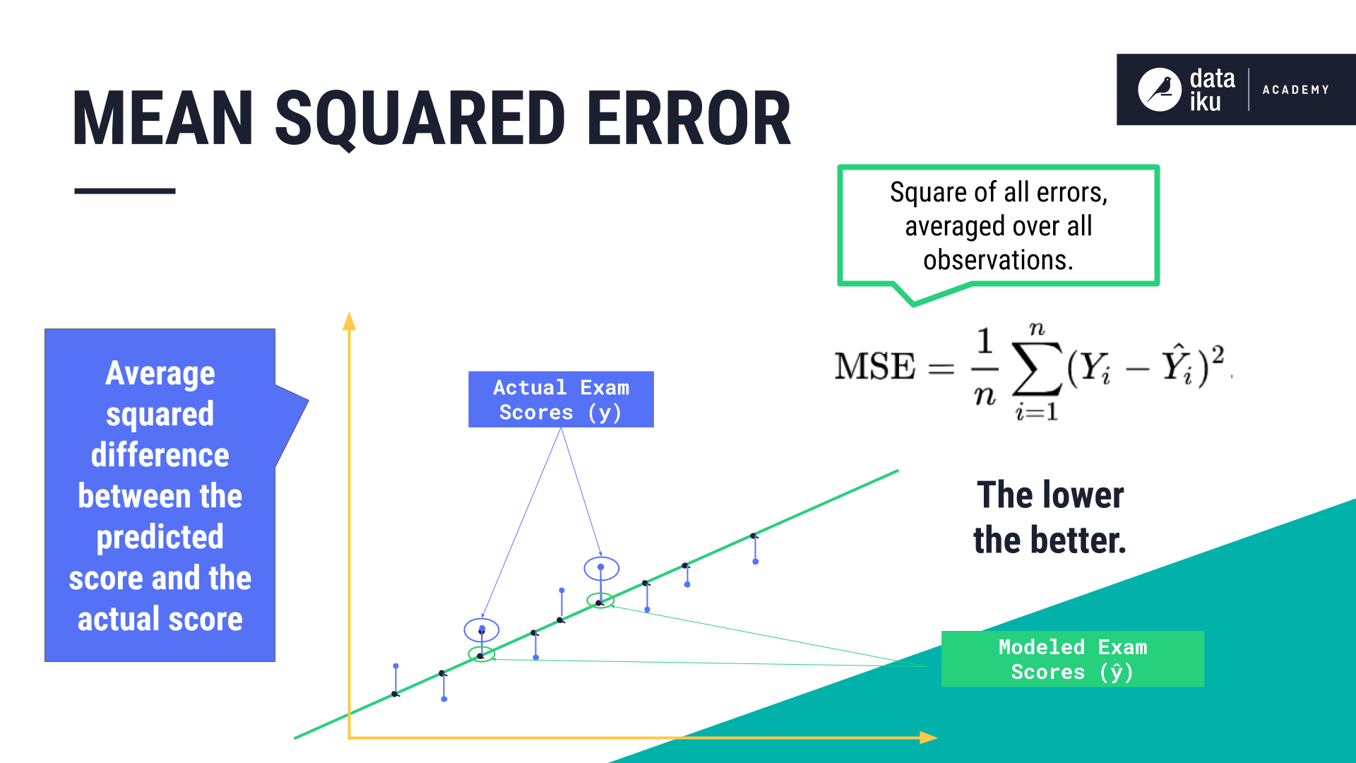
Mean squared error#
Mean squared error (MSE) is calculated by computing the square of all errors and averaging them over the number of observations.
The lower the MSE, the more accurate our predictions.
This metric measures the average squared difference between the predicted values and the actual values.
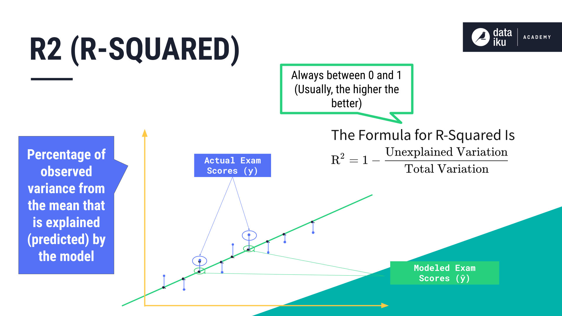
R-squared (R2)#
R2 is the percentage of the variance within the target variable that’s represented by the features in our model. A high R-squared, close to 1, indicates that the model fits the data well and frequently makes correct predictions.
Summary#
There are several metrics for evaluating machine learning models, depending on whether you are working with a regression model or a classification model.
In this lesson, we discovered some tools and metrics that we can use to evaluate our models. For example, we learned that a confusion matrix is a handy tool when trying to determine the threshold for a classification problem. We also learned that the TPR and FPR are used to create an ROC chart which is then used to create the AUC.
Next steps#
You can visit the other sections available in the course, Intro to Machine Learning and then move on to Machine Learning Basics.