Concept | Clustering algorithms#

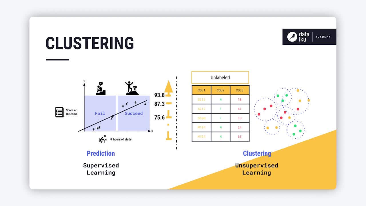
In prediction, or supervised learning, we are attempting to predict an outcome, such as whether or not a student will succeed on an exam, or the student’s exam score. In unsupervised learning, we have no labeled output. But the machine can still learn by inferring underlying patterns from an unlabeled dataset. The most common method of unsupervised learning is clustering.

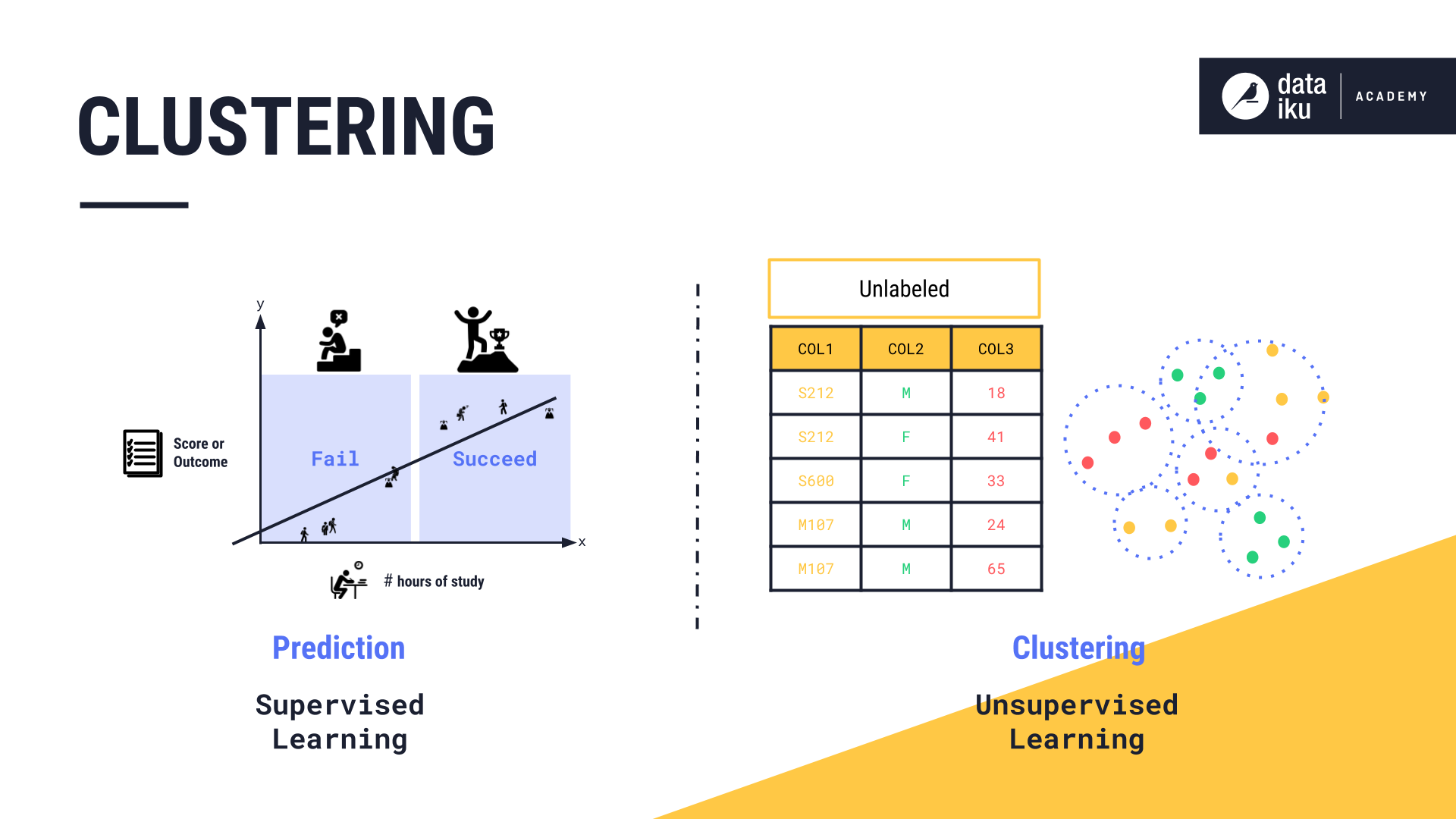
A clustering algorithm aims to detect patterns and similarities in the dataset.

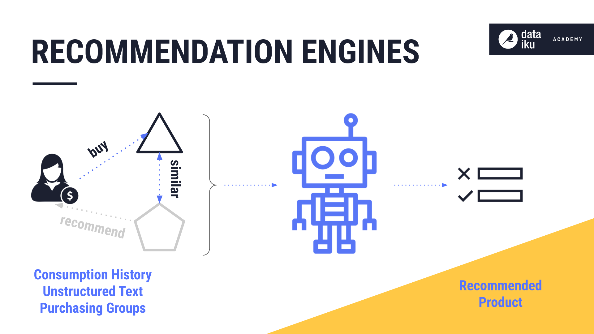
One popular use case for clustering is recommendation engines, which are systems built to predict what users might like, such as a movie or a book.

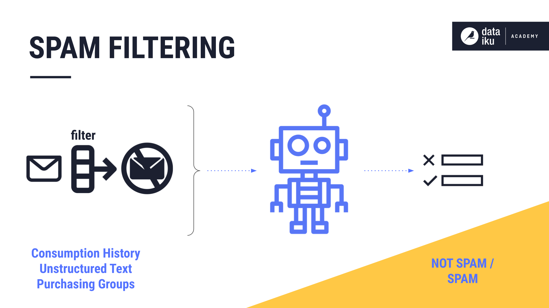
Another use case for clustering is spam filtering where emails that have been identified as spam end up in the junk folder of an inbox.

In this lesson, we will learn about two common methods of cluster analysis: K-Means and hierarchical clustering.

In K-Means, we aim to set K to an optimal number, creating just the right number of clusters where adding more clusters would no longer provide a sufficient decrease in variation.
In hierarchical clustering, we aim to first understand the relationship between the clusters visually, and then determine the number of clusters, or hierarchy level, that best portrays the different groupings.

Let’s look at each of these methods in more detail.

K-Means#

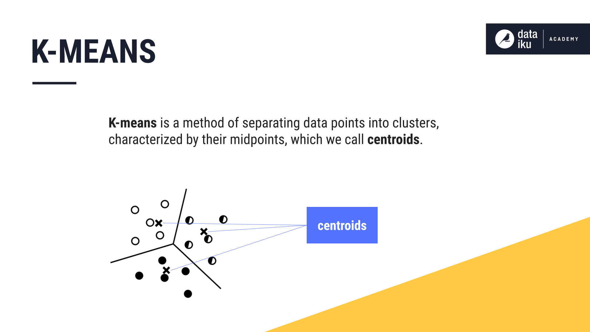
K-Means separates data points into clusters, characterized by their midpoints, which we call centroids.

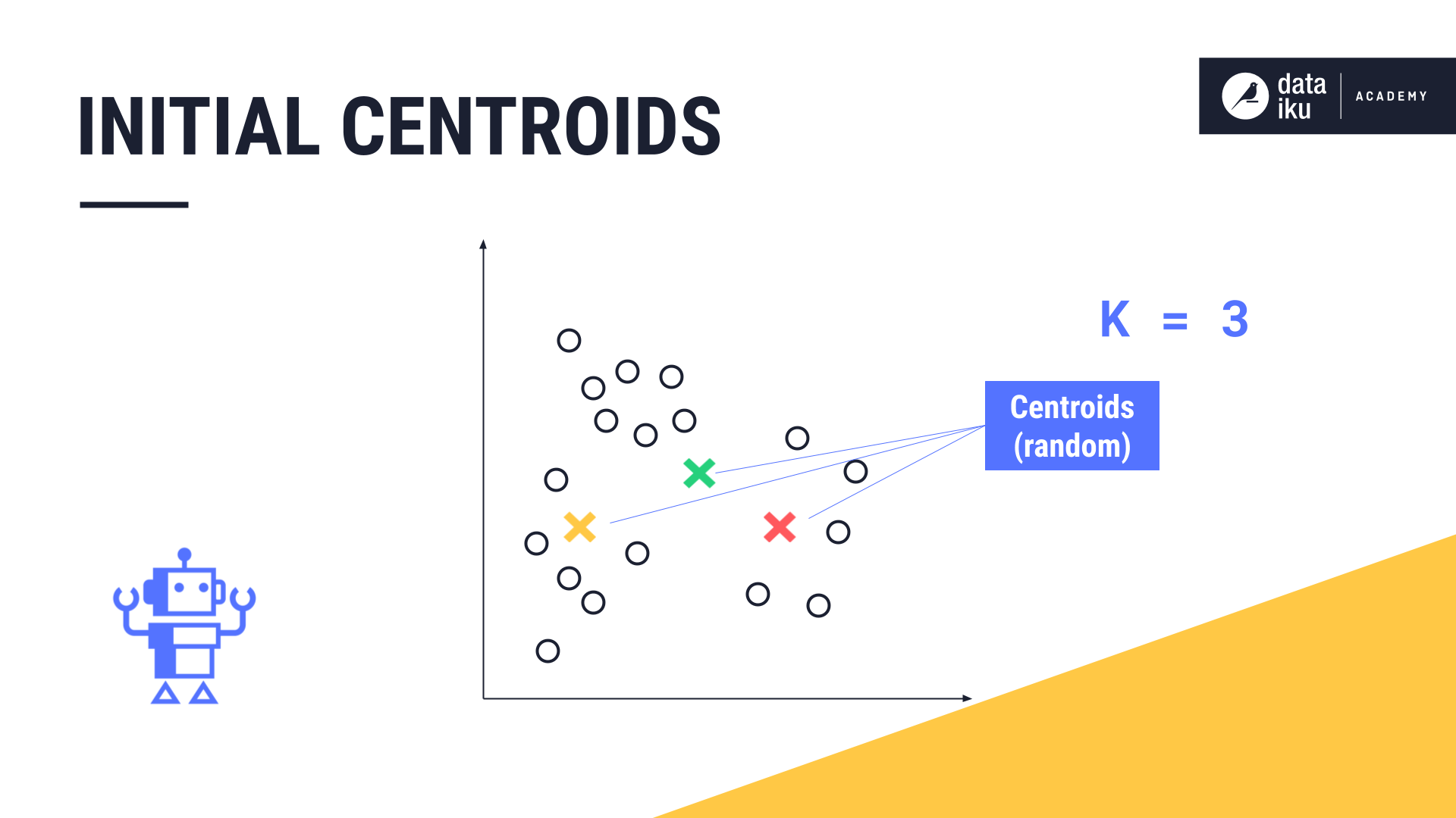
Let’s use an example to demonstrate K-Means. To begin, we select “K”, or the number of clusters that we want to identify in our data. For our example, K is equal to three. This means we will identify three clusters in our data.

First, K-Means takes this number, three, and marks three random points on the chart. These are the centroids, or midpoints, of the initial clusters.

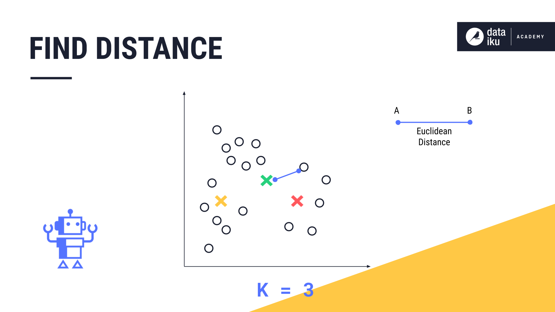
Next, K-Means measures the distance, known as the euclidean distance, between each data point and each centroid.

Finally, it assigns each data point to its closest centroid and the corresponding cluster.

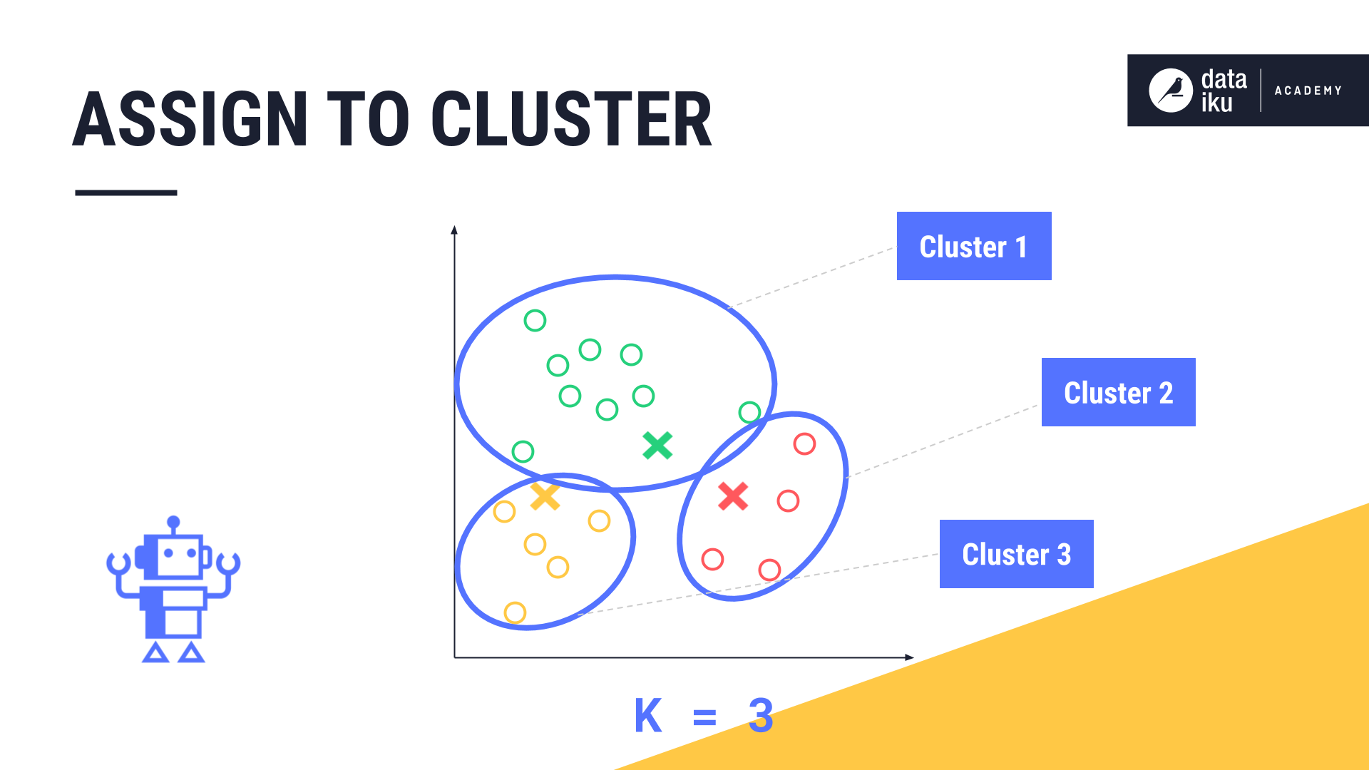
Once each data point is assigned to these initial clusters, the new midpoint, or centroid, of each cluster is calculated.

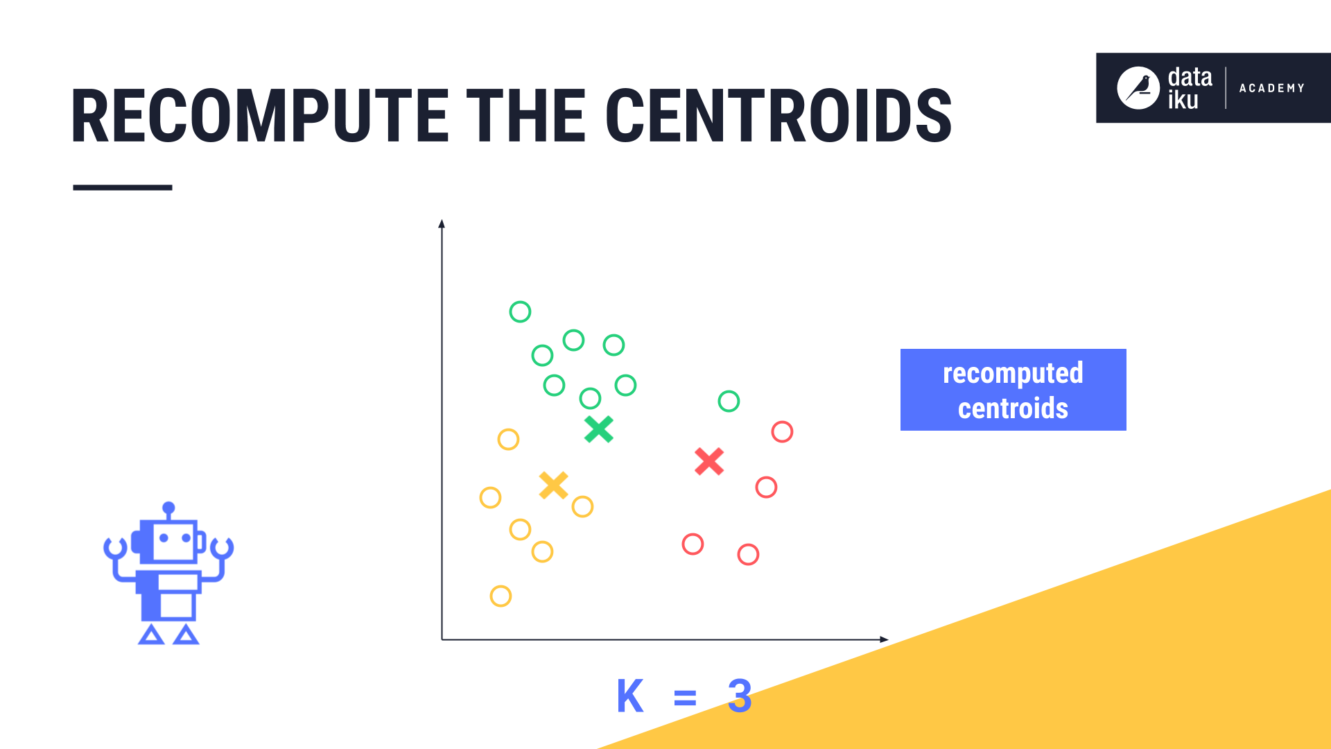
K-Means repeats the steps of measuring the euclidean distance between each data point and the centroid, re-assigning each data point to its closest centroid, and then calculating the new midpoint of each cluster again.

This continues until one of two outcomes occurs: either the clusters stabilize, meaning no data points can be reassigned, or, a predefined maximum number of iterations has been reached.

Elbow plot#

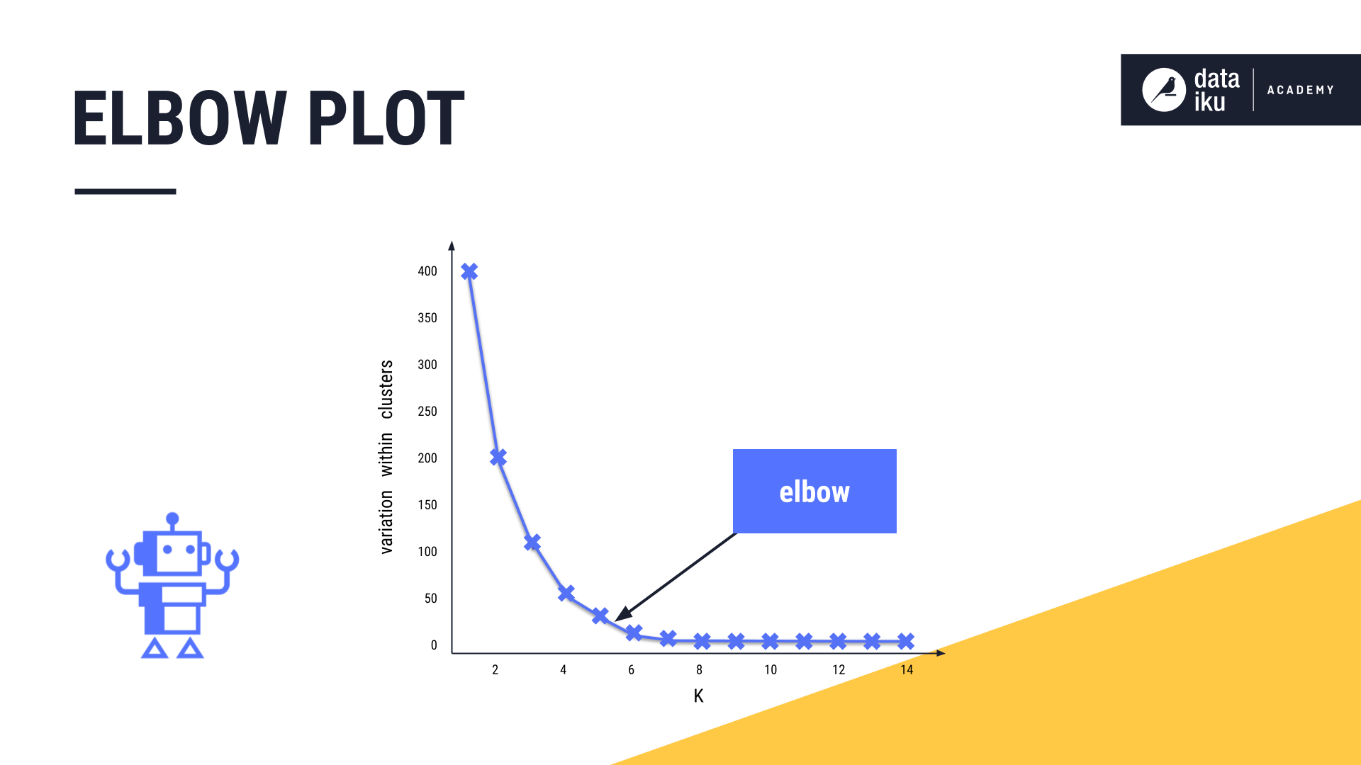
In K-Means, we want to set K to an optimal number, creating just the right number of clusters. The most common method for determining the optimal value for K is to use an elbow plot.

The goal of the elbow plot is to find the elbow, or the inflection point of the curve. This is where increasing the value of K, or adding more clusters, is no longer providing a sufficient decrease in variation.

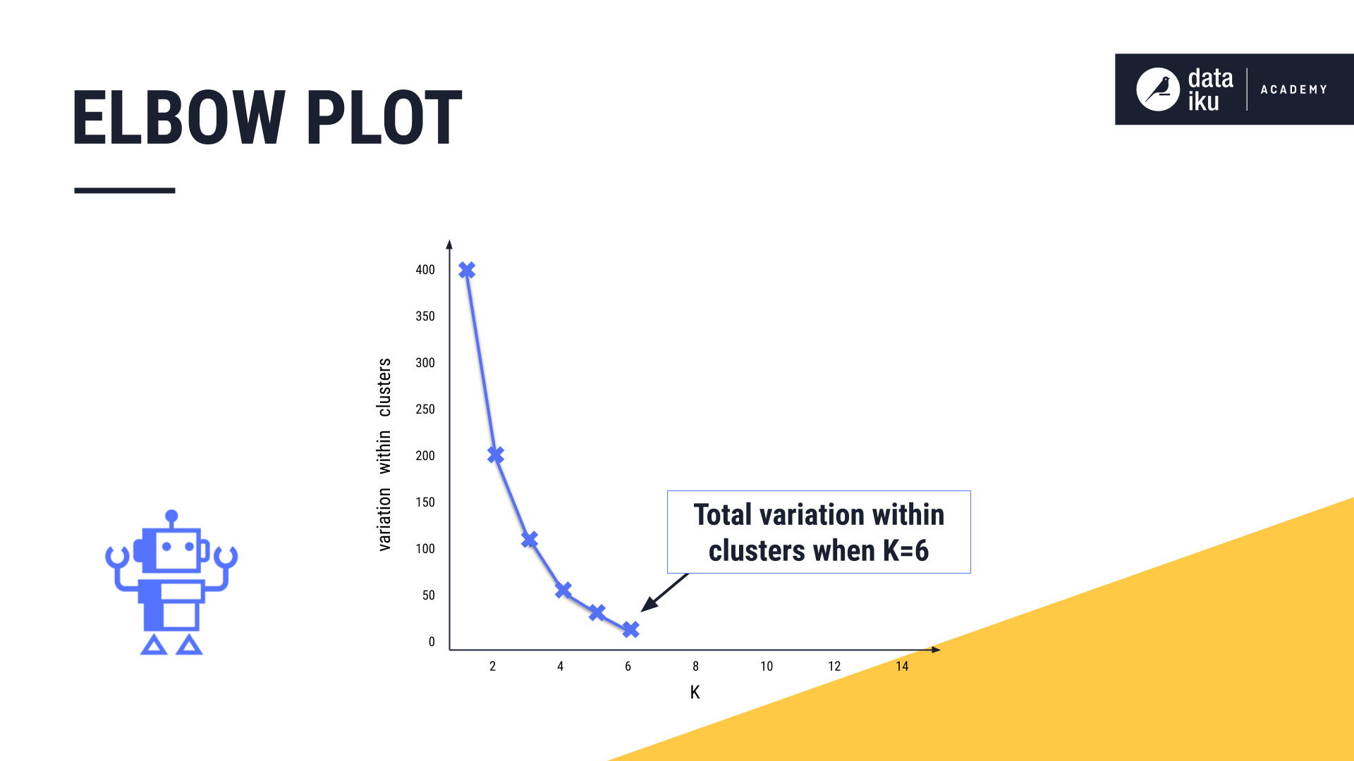
To build our elbow plot, we iteratively run the K-Means algorithm, first with K=1, then K=2, and so forth, and computing the total variation within clusters at each value of K.

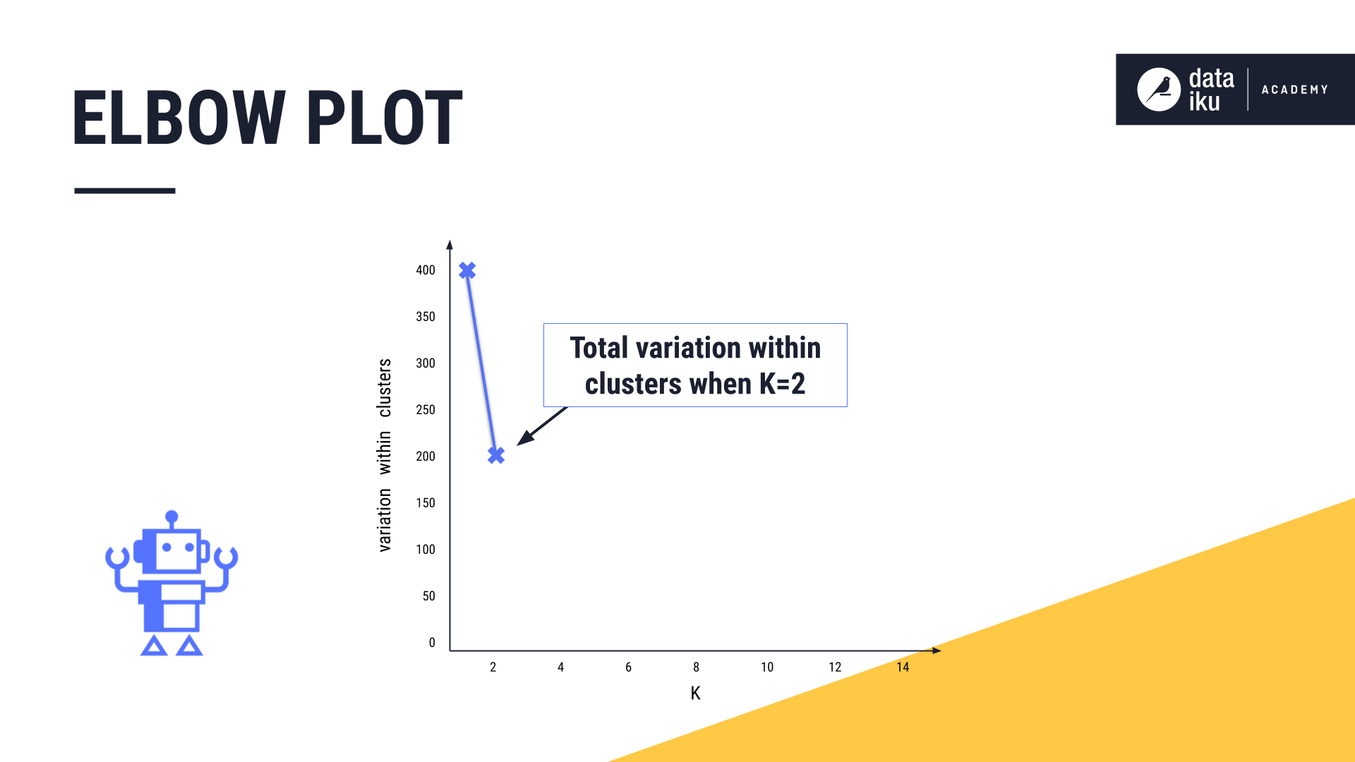
As we increase the value of K and the number of clusters increases, the total variation within clusters will always decrease, or at least remain constant.

In our example, the elbow is approximately “five”, so we may want to opt for five clusters.

Hierarchical clustering#

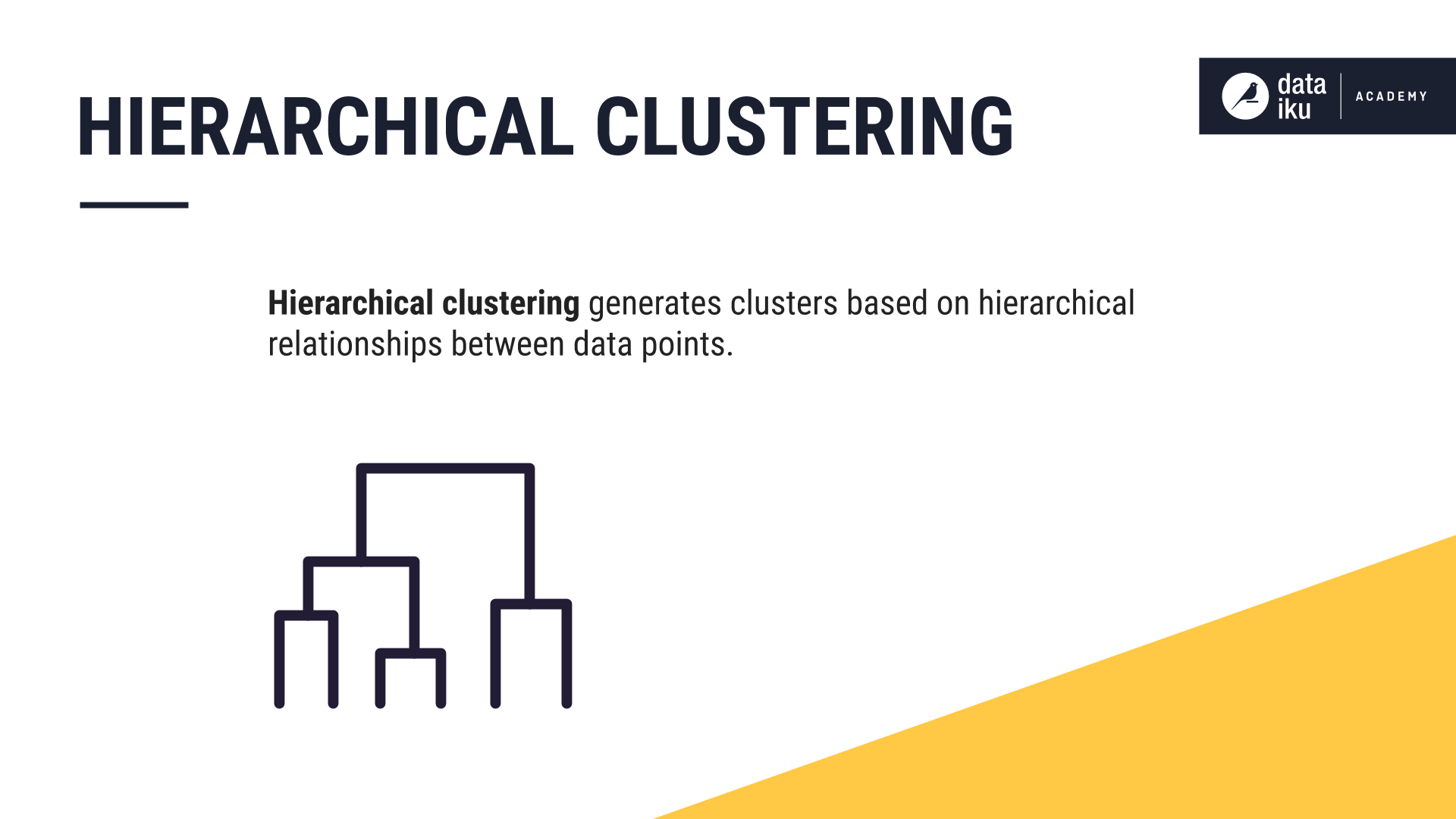
Let’s look at another common clustering method, hierarchical clustering. Hierarchical clustering generates clusters based on hierarchical relationships between data points.

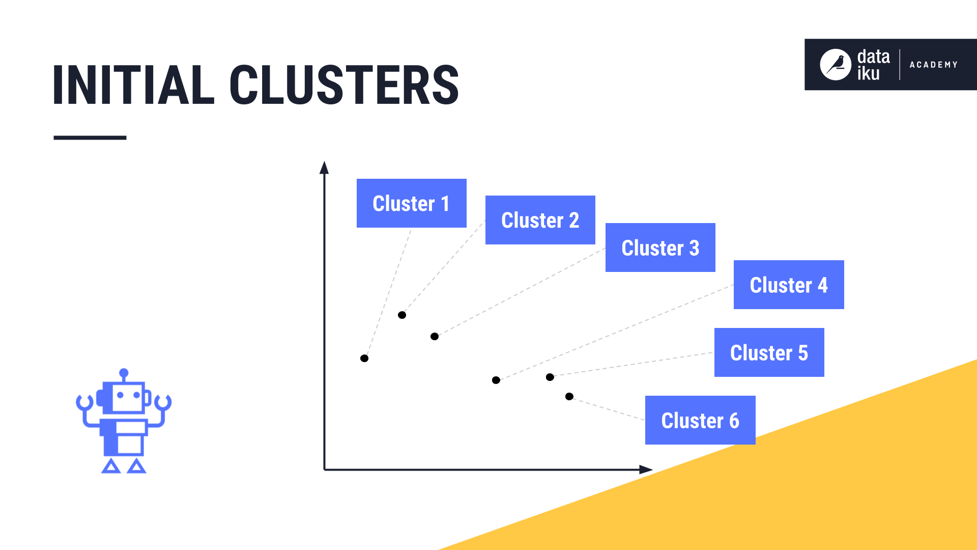
In this method, instead of beginning with a randomly-selected value of “K”, hierarchical clustering starts by declaring each data point as a cluster of its own.

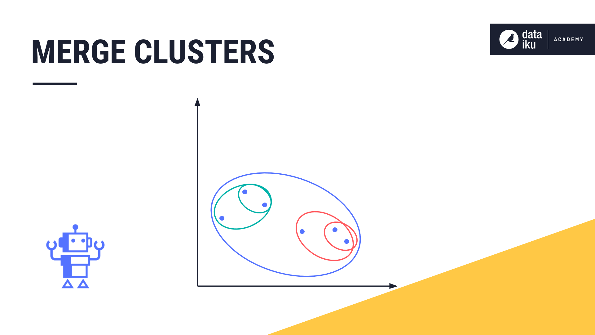
Then, hierarchical clustering computes the euclidean distance between all cluster pairs.

Next, the two closest clusters are merged into a single cluster. Hierarchical clustering iteratively repeats this process until all data points are merged into one large cluster.

Dendrogram#

To visualize the hierarchical relationship between the clusters and determine the optimal number of clusters for our use case, we can use a dendrogram. A dendrogram is a diagram that shows the hierarchical relationship between objects.

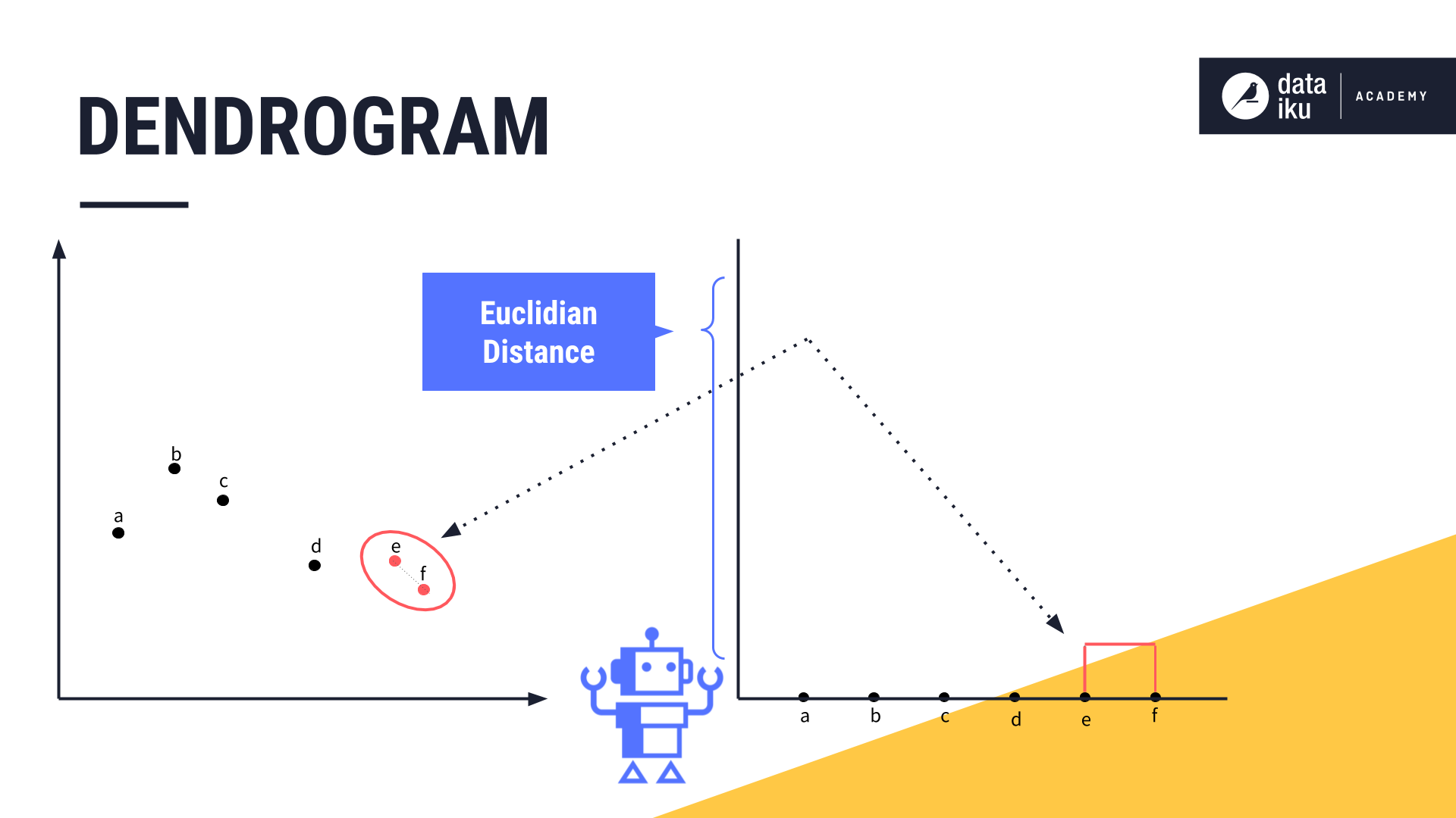
To build our dendrogram, we name each of our data points, declaring each one as its own cluster.

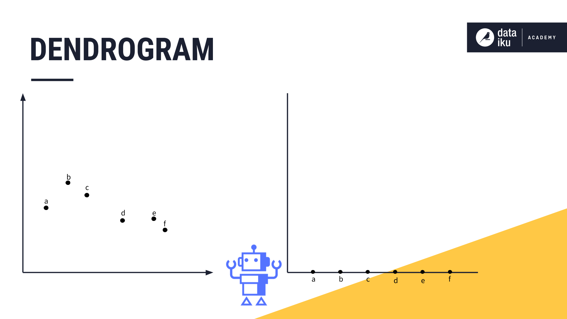
Then we iteratively combine the closest pairs. Points “E” and “F” are the first to be merged, so we draw a line linking these two data points in our dendrogram. The height of that line will be determined by the distance between these two data points on the original chart.

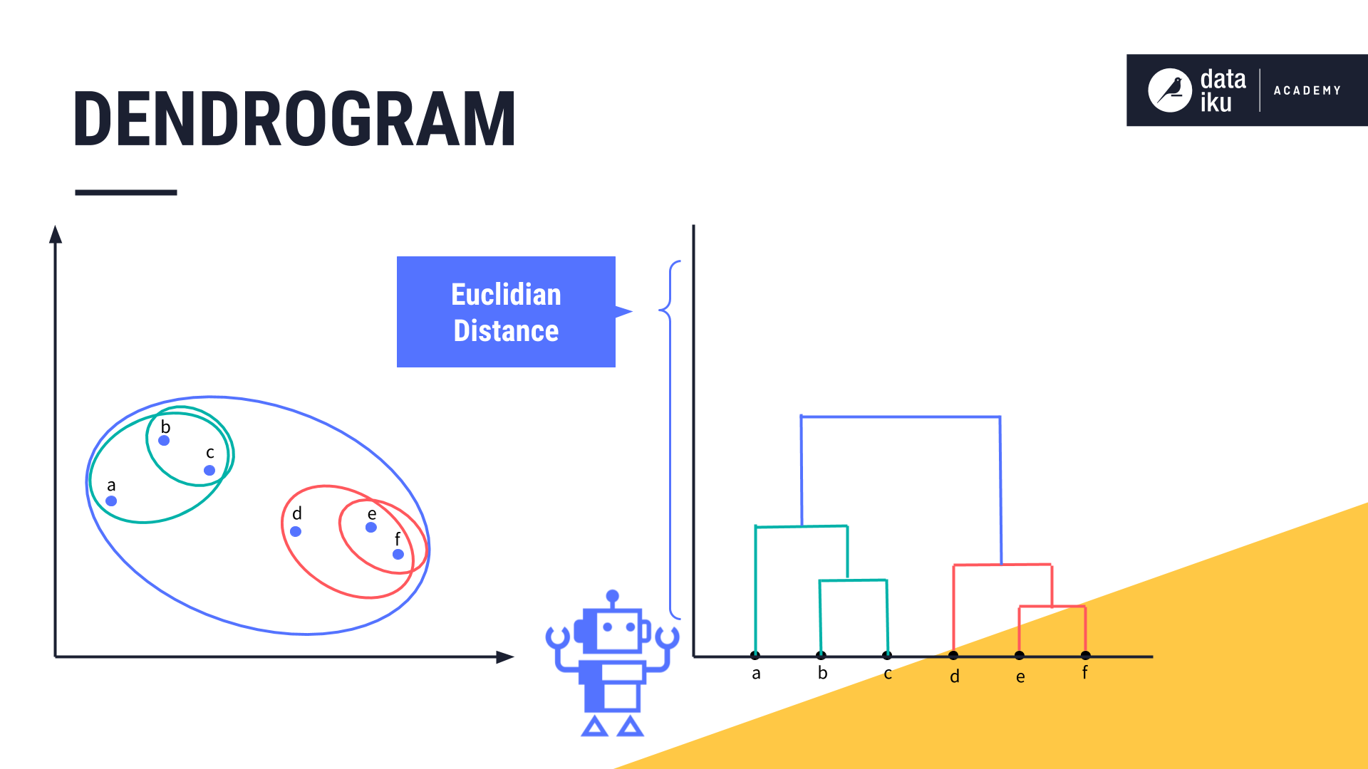
We continue merging the next two closest clusters, and so forth, and adding the relevant lines to the chart.

Let’s now use our dendrogram to help determine the optimal number of clusters. Based on our knowledge of the business domain and the use case, we can set a distance threshold, also known as a cluster dissimilarity threshold. We can use this horizontal line to see how many clusters we’d have at this threshold by counting how many vertical lines it bisects.

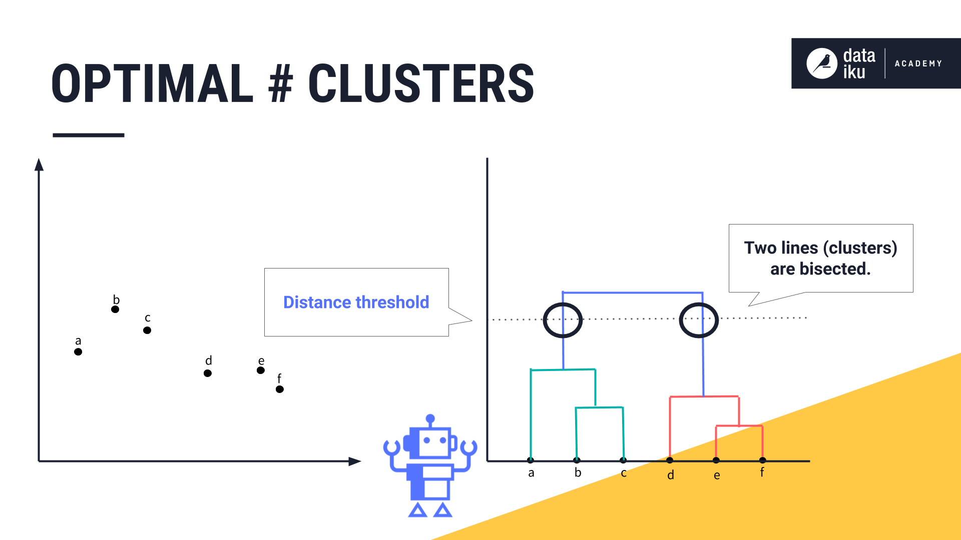
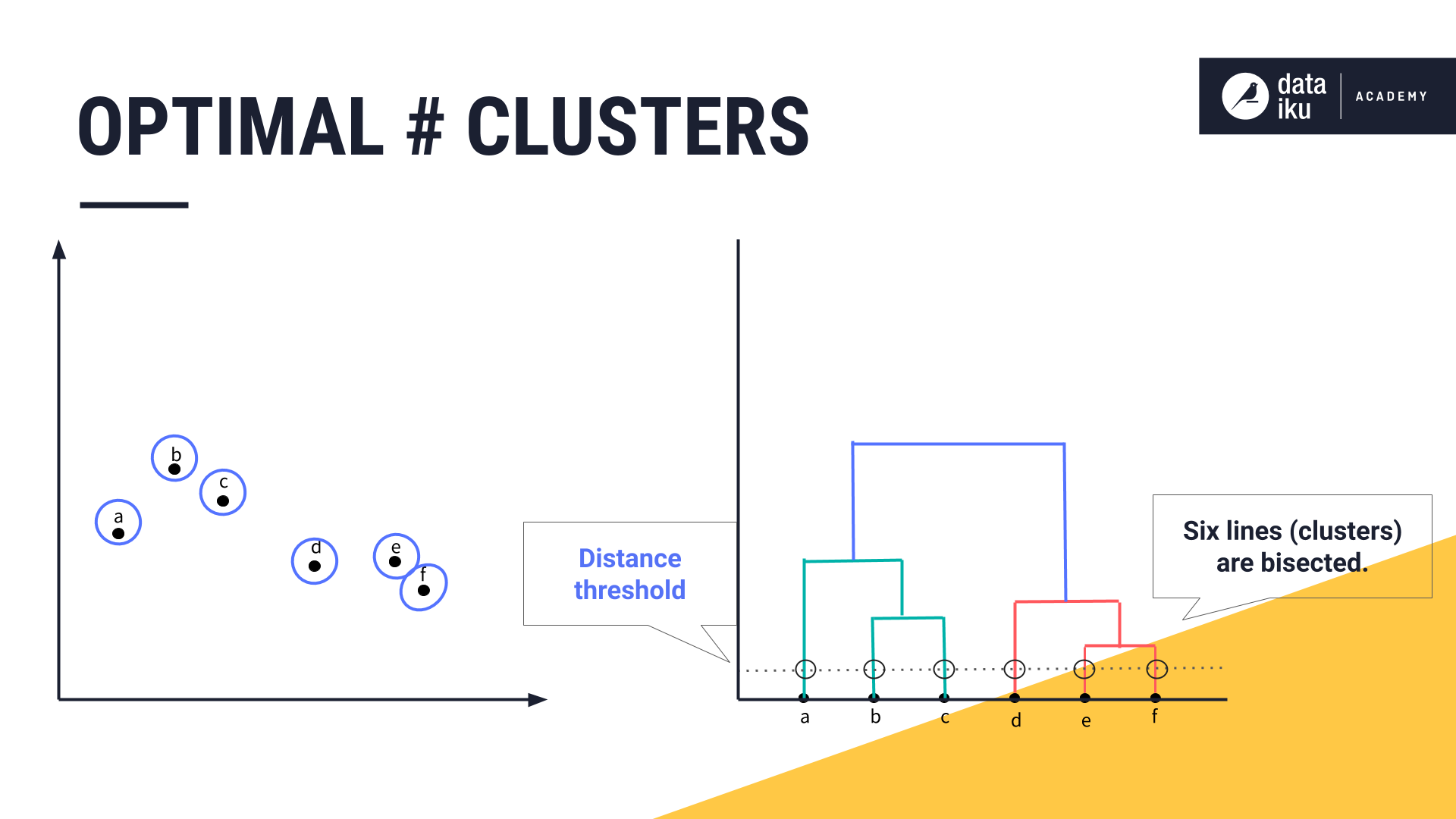
Depending on our use case, we might decide one cluster would contain points A, B and C, and the other would contain points D, E, and F. Alternatively, we might decide that our clusters must be as dissimilar as possible. In our case, if we set the distance threshold so that each cluster is as dissimilar as possible, we would have six bisected lines, resulting in six clusters.

What’s next?#

You can visit the other sections available in the course, Intro to Machine Learning and then move on to Machine Learning Basics.

For a quick read about clustering, check out the Dataiku blog post, Clustering: How It Works (In Plain English!).