
Tutorial | Column-based partitioning#
Get started#
In this tutorial, we will modify a completed Flow dedicated to the detection of credit card fraud. Our goal is to be able to predict whether a transaction is fraudulent based on the transaction subsector (such as insurance, travel, or gas) and the purchase date.
Objectives#
Our Flow should meet the following business objectives:
Be able to create time-based computations.
Train a partitioned model to test the assumption that fraudulent behavior is related to merchant subsector, which is discrete information.
To meet these objectives, we will work with both discrete and time-based partitioning. Specifically, by the end of the lesson, we will accomplish the following tasks:
Partition a dataset for the purpose of optimizing a flow and creating targeted features.
Create the following partitions:
Time-based partitioning. We will partition by purchase date for the purpose of targeting a specific date.
Discrete partitioning. We will partition by subsector (for example, internet, gas, or travel) for the purpose of targeting a specific subsector.
Propagate partitioning in a Flow.
Stop partitioning in a Flow, collecting the partitions.
Prerequisites#
Dataiku 12.0 or later.
An SQL connection. For an overview of which databases are supported by Dataiku, see Other SQL databases in the reference documentation.
Create the project#
From the Dataiku Design homepage, click + New Project.
Select Learning projects.
Search for and select Partitioning: Column-Based.
If needed, change the folder into which the project will be installed, and click Create.
From the project homepage, click Go to Flow (or type
g+f).
Note
You can also download the starter project from this website and import it as a ZIP file.
Use case summary#
The Flow contains the following datasets:
cardholder_info contains information about the owner of the card used in the transaction process.
merchant_info contains information about the merchant receiving the transaction amount, including the merchant subsector (subsector_description).
transactions_ contains historical information about each transaction including the purchase_date.
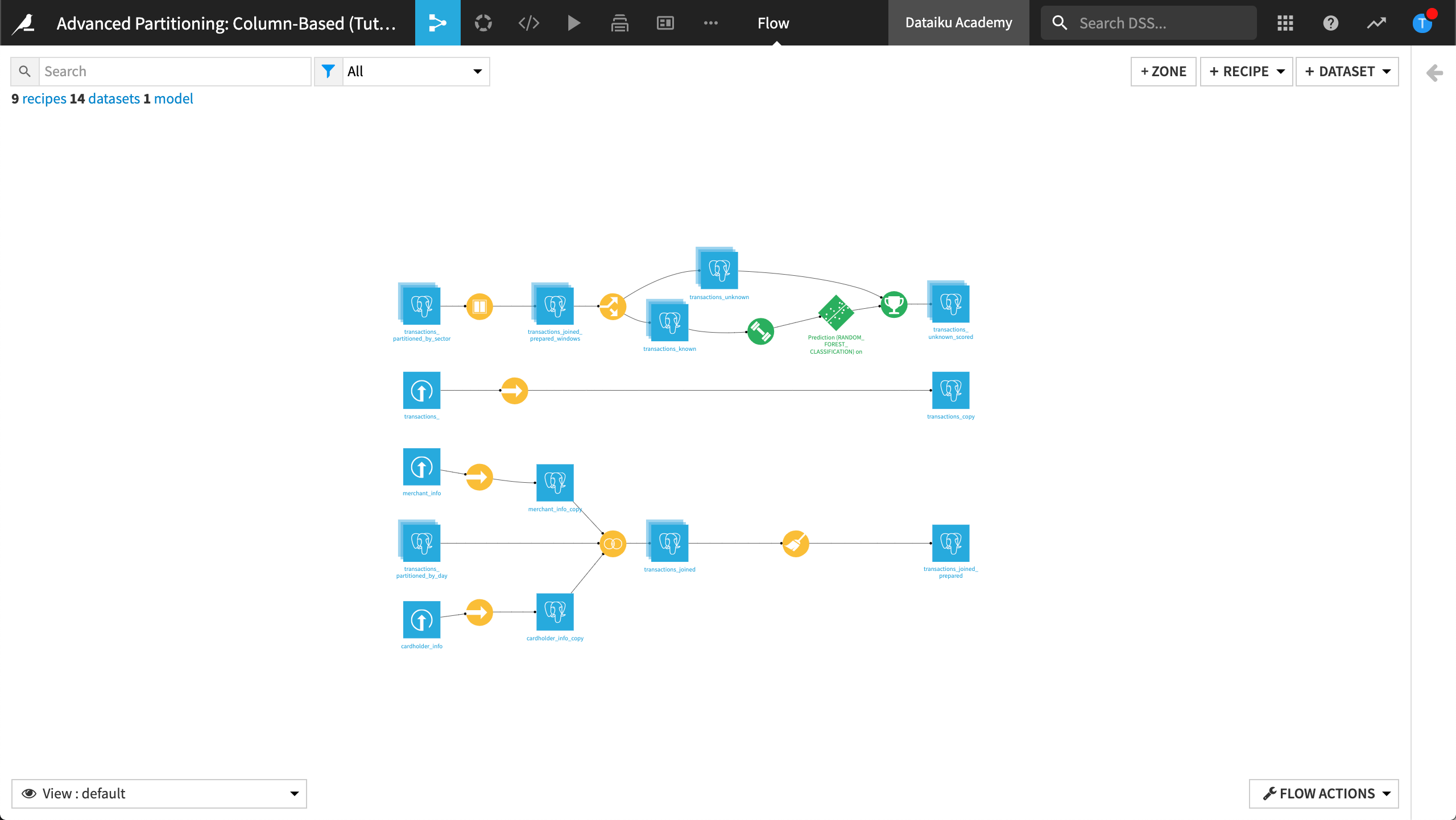
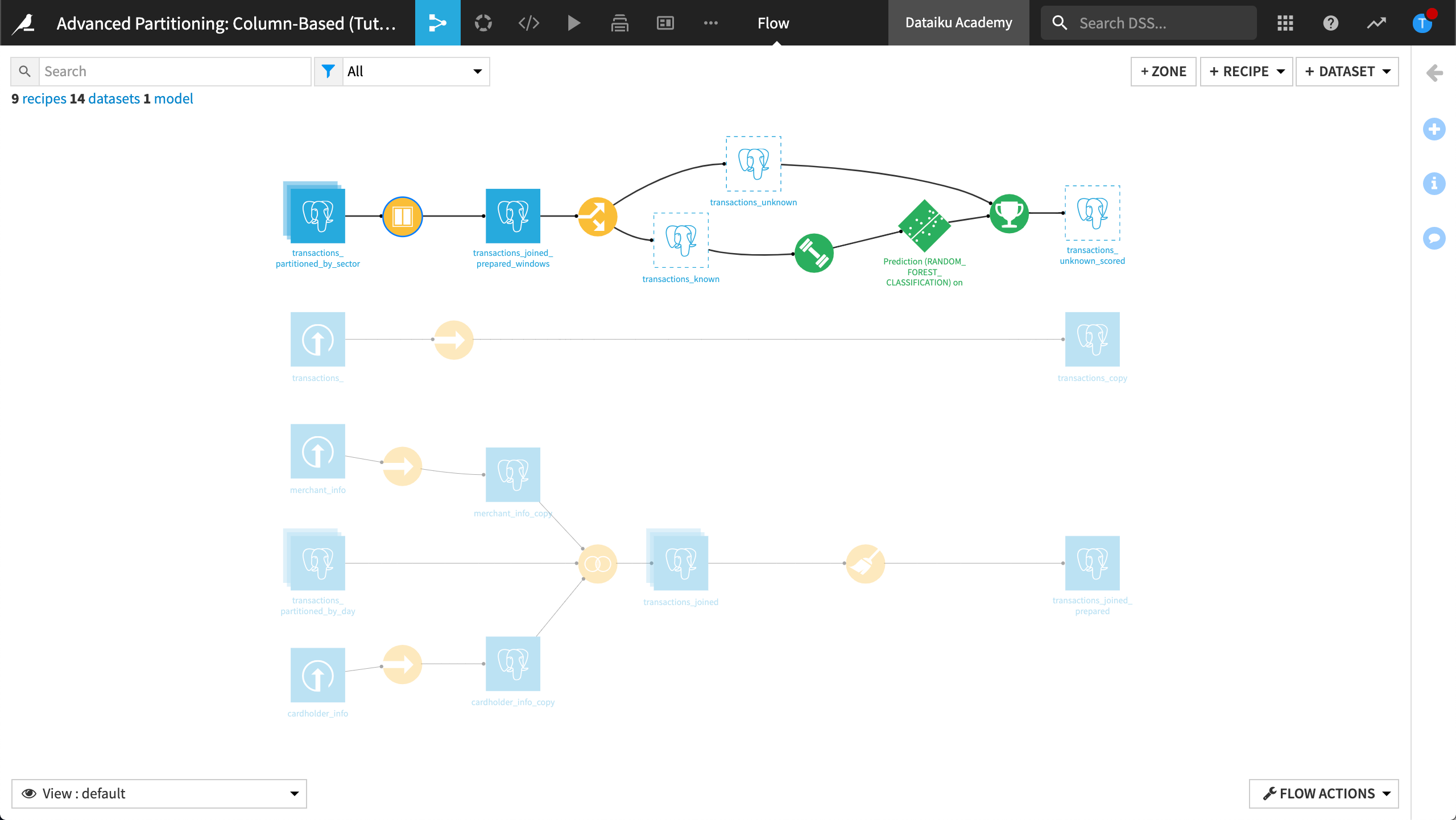
The final pipeline in Dataiku is shown below.
Change the dataset connections#
To work with column-based partitioning, our datasets must have an SQL connection. In this step, we will change the connections of all our datasets from the local filesystem to the SQL connection defined on your Dataiku instance.
Go to the Flow.
Select all datasets except for the initial input datasets.
Open the right panel, then click Change connection.
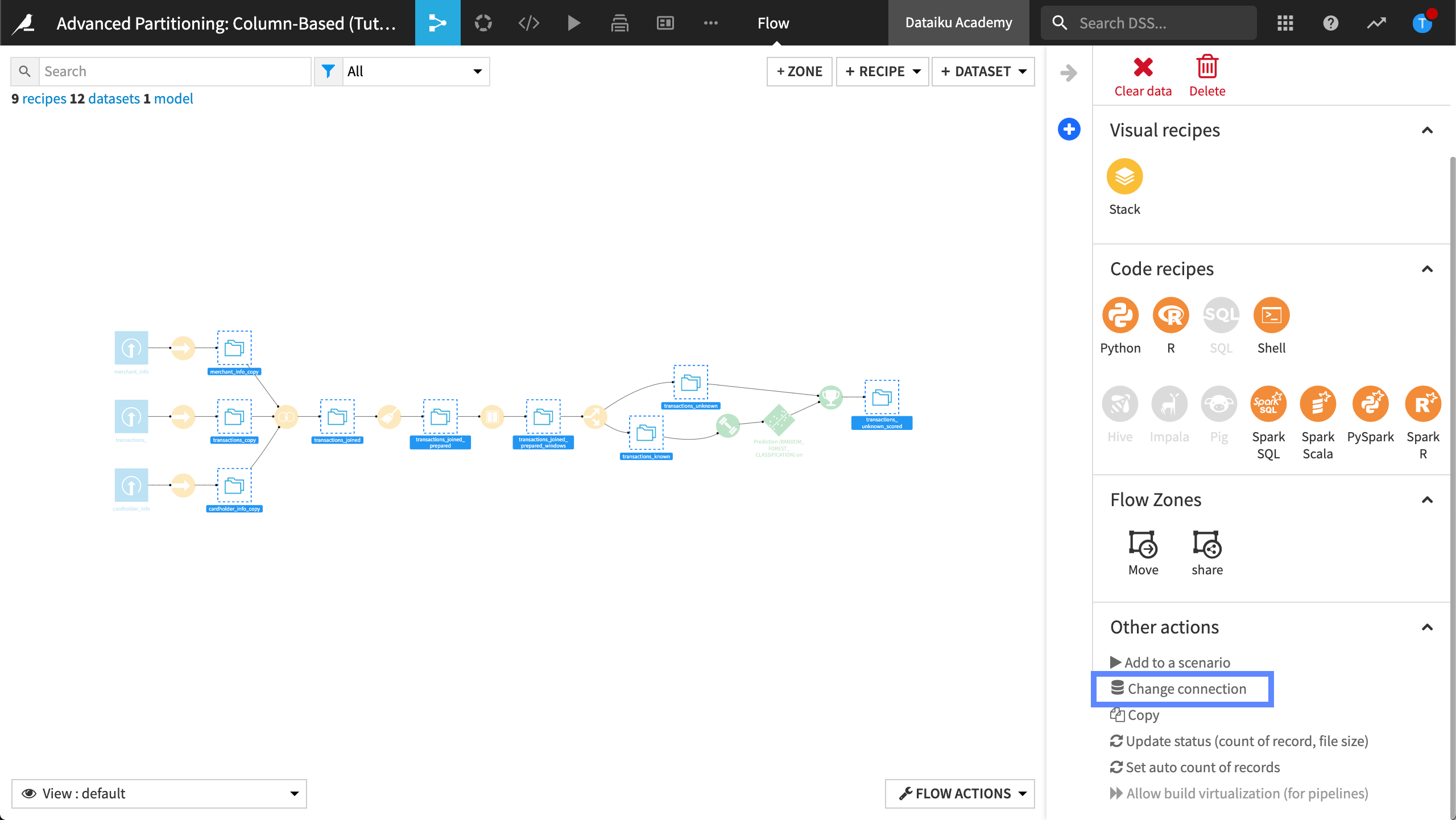
Dataiku displays the change connection dialog box.
In New connection, select your SQL connection.
Select Drop data. We won’t need the filesystem datasets.
Click Save.
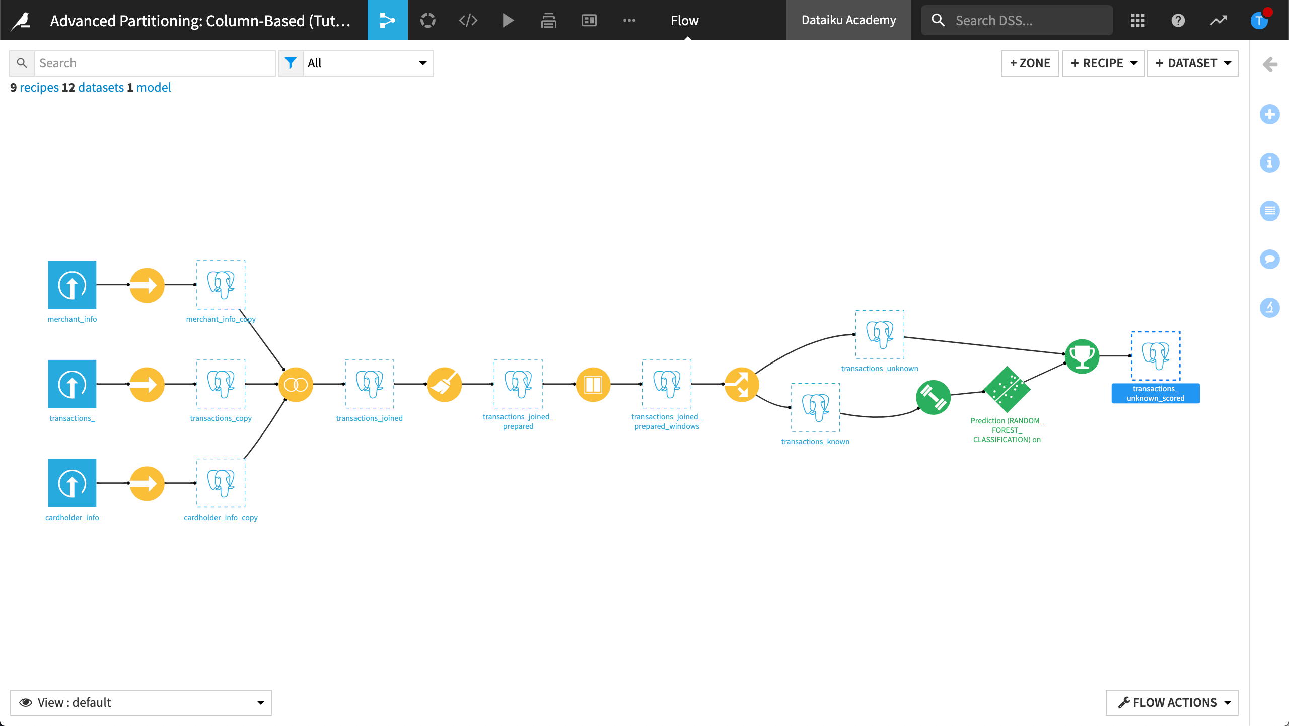
The Flow looks like this:
Build a time-based partitioned dataset#
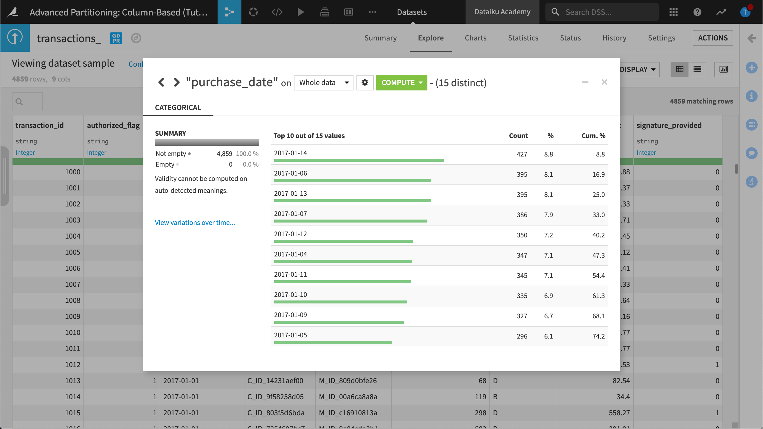
In this section, we will partition the dataset, transactions_copy, using the purchase_date dimension. The column, purchase_date, contains values representing the date of the credit card transaction. For the purposes of this tutorial, the number of distinct purchase dates has been limited to 15 values.
Create a partitioned output#
In this section, we will create a partitioned dataset, transactions_partitioned_by_day, without duplicating the data. To do this, we will create a new logical pointer to the same SQL table.
Create transactions_partitioned_by_day#
Run the Sync recipe that was used to create transactions_copy so that the dataset is built.
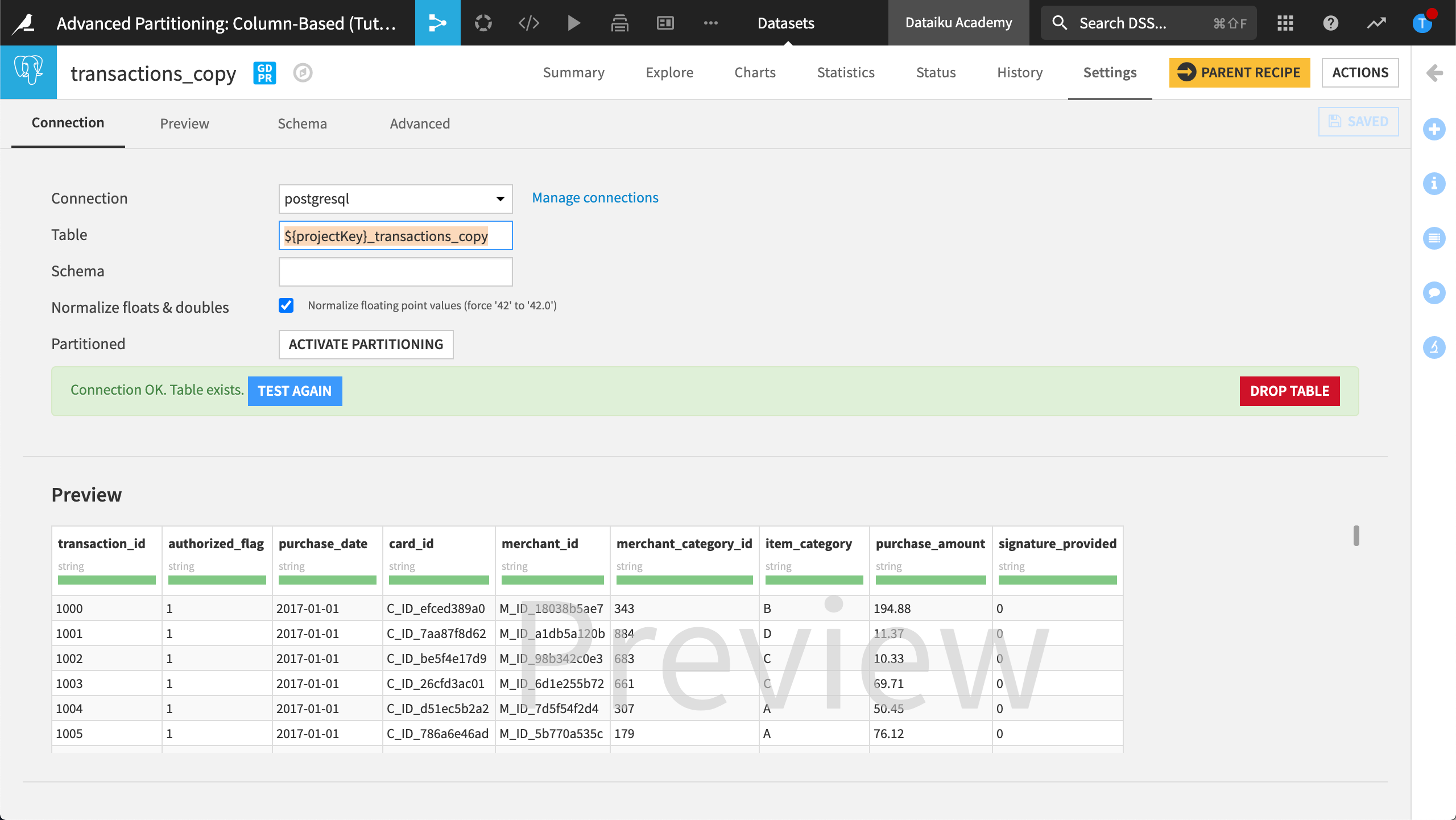
Open transactions_copy and view the Settings page.
Copy the contents of the Table and Schema fields, then save the information for later.
Return to the Flow.
In the upper-right-hand corner, click +Dataset.
From the SQL databases menu, select your SQL connection.
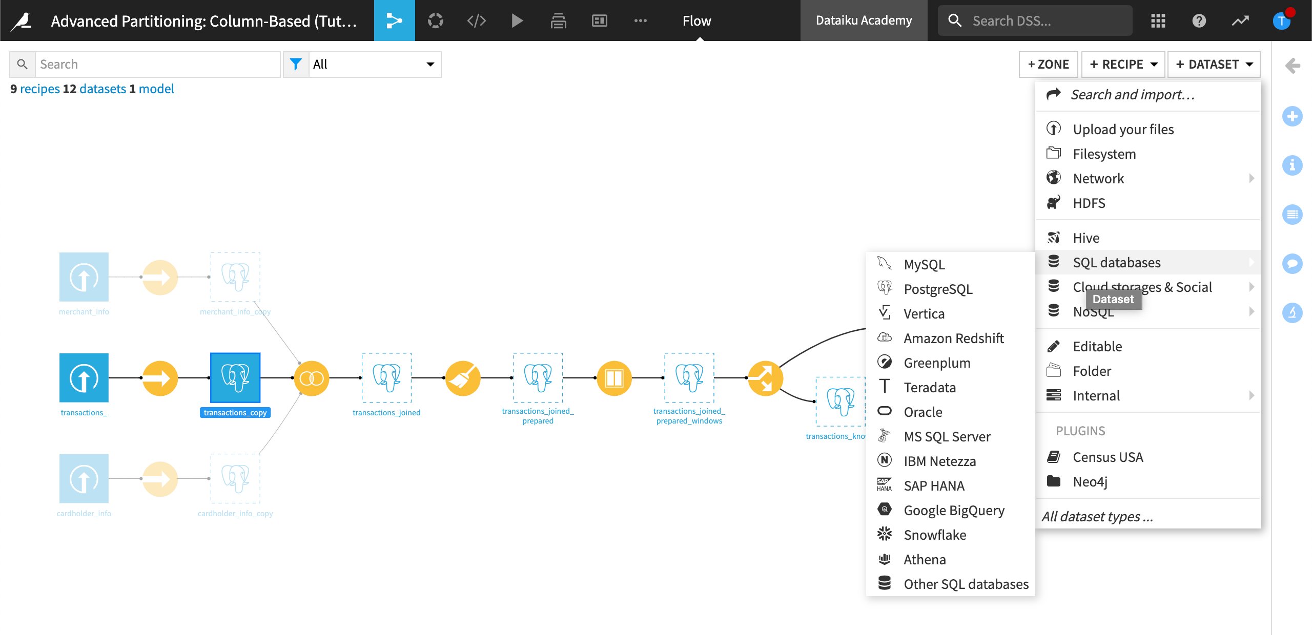
Dataiku displays the configuration page for the SQL connection you selected.
Paste the information you saved into the Table and Schema fields.
Click Test Table.
Note
If the table is undefined, you can locate it by getting the list of tables.
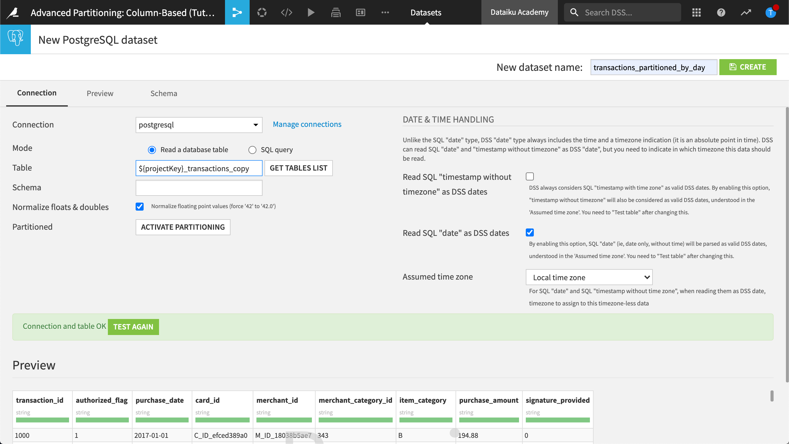
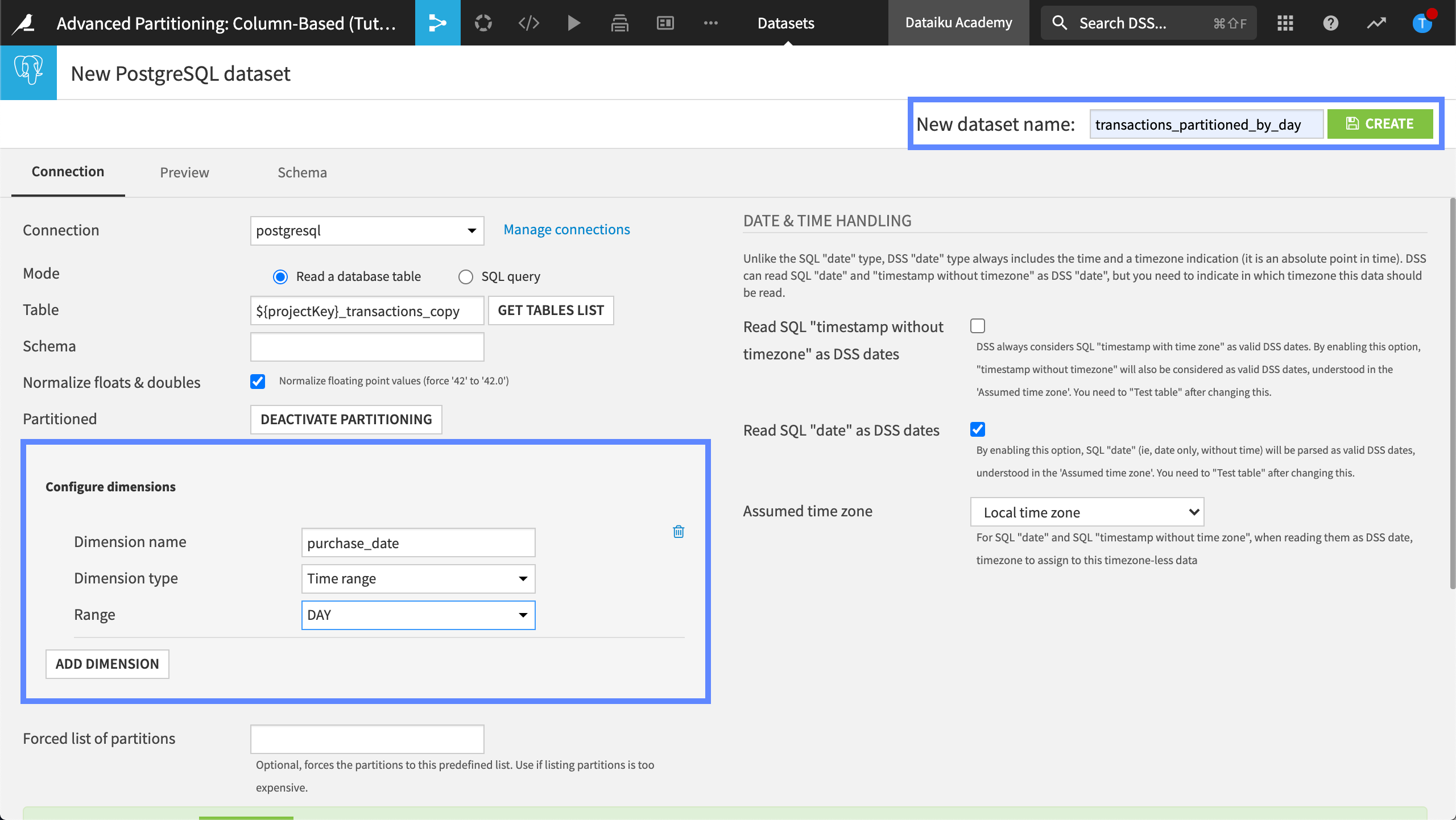
Next to Partitioned, click Activate Partitioning to enable column-based partitioning for this SQL dataset.
Configure the dimension as follows:
Name the dimension,
purchase_date.Set the dimension type to Time range.
Set the range to Day.
Let’s create this dataset.
In the upper-right-hand corner, name the new dataset,
transactions_partitioned_by_day.Click Create.
Configure the Join recipe#
Configure the Join recipe to change the input dataset from transactions_copy to transactions_partitioned_by_day:
Run the Sync recipe that was used to create merchant_info_copy.
Run the Sync recipe that was used to create cardholder_info_copy.
Open the Join recipe that was used to create transactions_joined.
Click to replace the transactions_copy dataset.
Replace the transactions_copy dataset with transactions_partitioned_by_day.
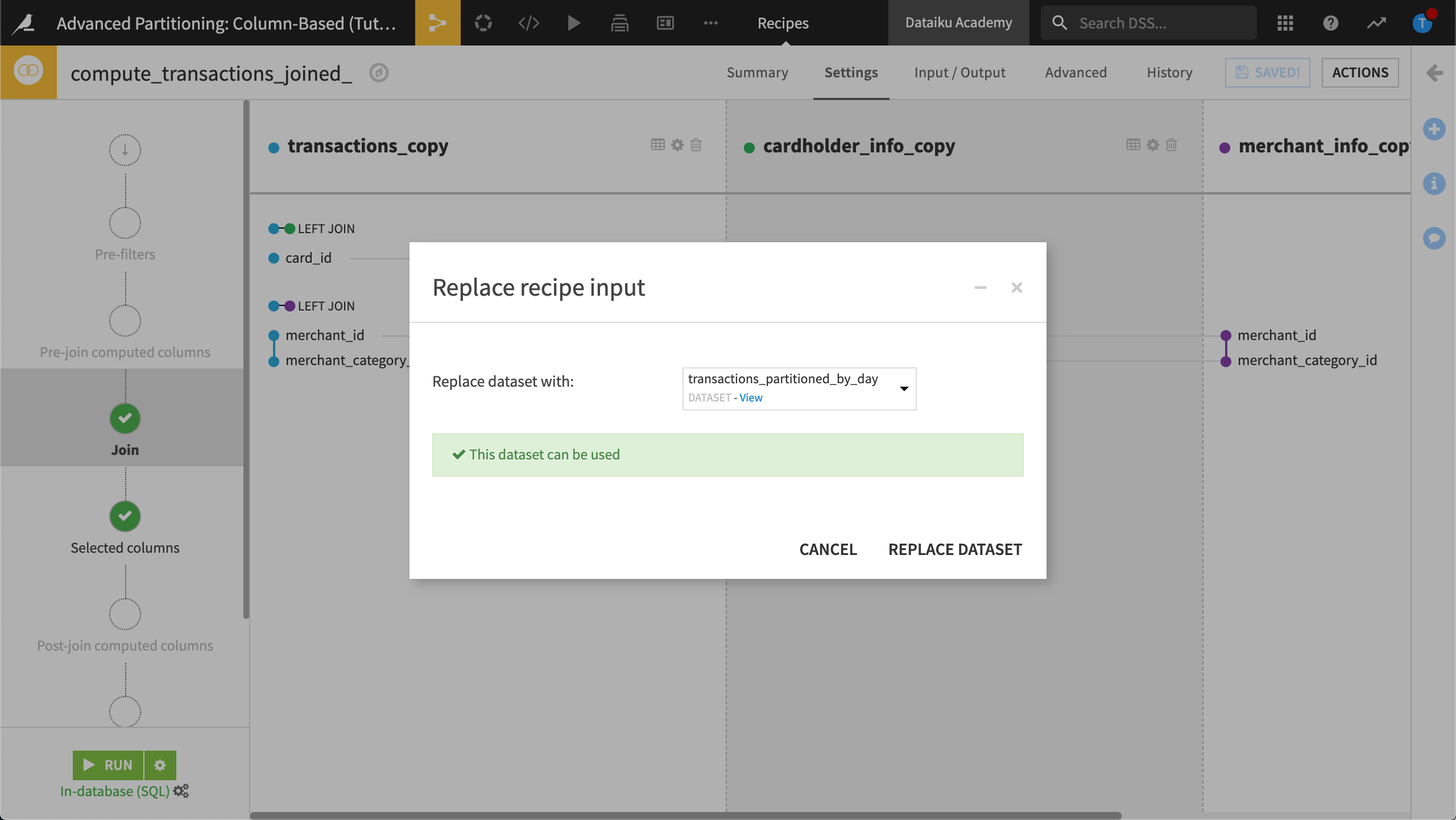
Click Replace Dataset.
In the Input / Output tab, set the partition dependency function type to All available.
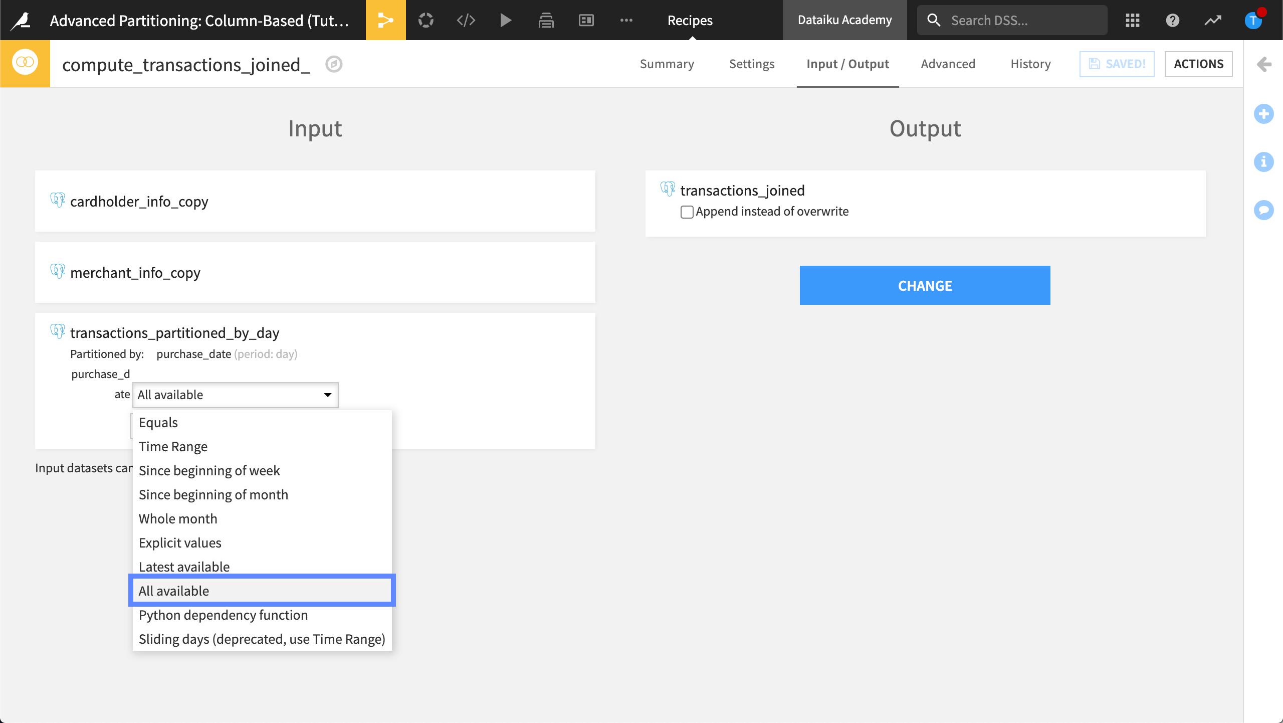
Save and run the recipe.
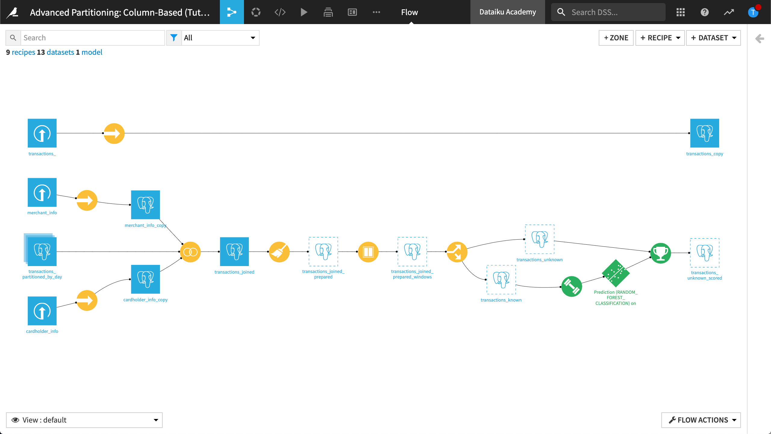
Return to the Flow.
Our Flow now looks like this:
Propagate the time-based partition dimension across the Flow#
Now that our dataset is partitioned, we can propagate the partitioning dimension across the Flow.
Partition the transactions_joined dataset#
Partition transactions_joined and identify the partition dependencies using the following steps:
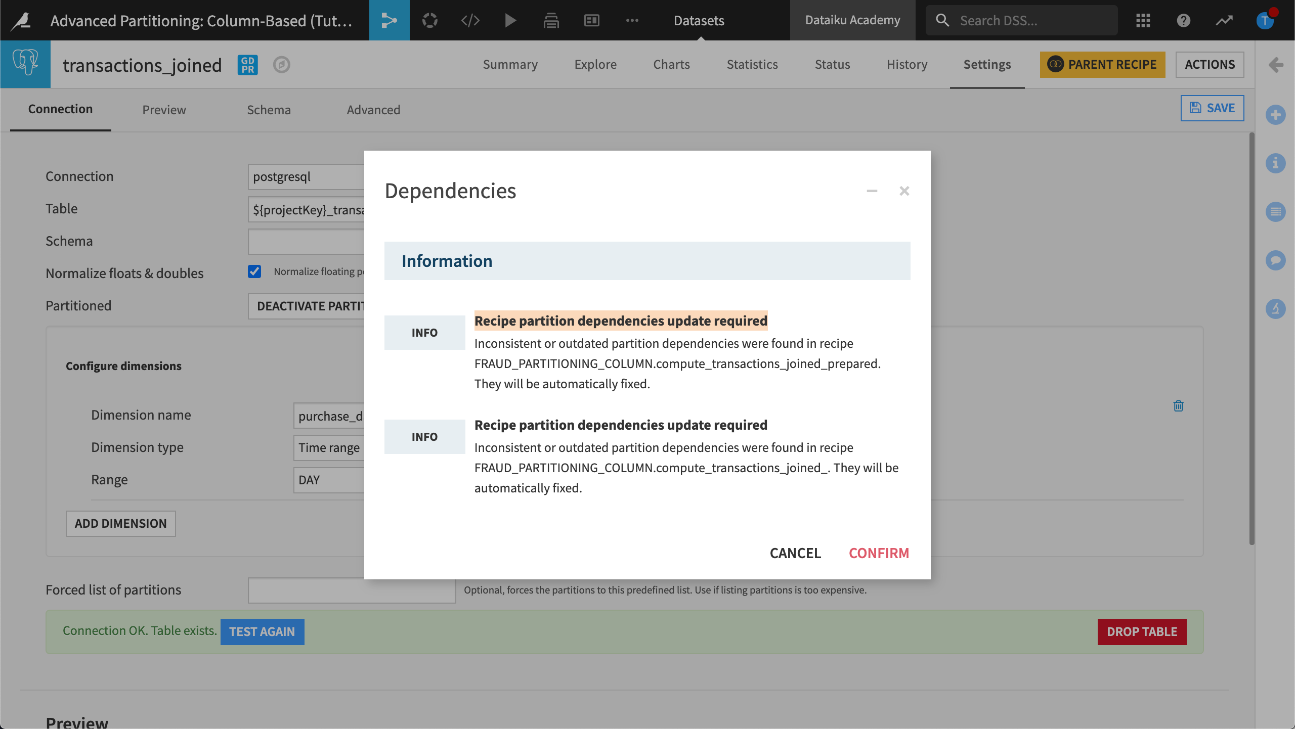
Open the transactions_joined dataset.
View Settings > Connection.
Click Activate Partitioning.
Configure the dimension as follows:
Name the dimension,
purchase_date.Set the dimension type to Time range.
Set the range to Day.
Click Save and click Confirm to confirm that dependencies with this dataset will be changed.
The datasets transactions_partitioned_by_day and transactions_joined are now both partitioned by the purchase_date dimension.
Identify the partition dependencies#
Now we must identify which partition dependency function type (All available, Equals, Time Range, etc.) we want to map between the two datasets transactions_partitioned_by_day and transactions_joined.
To do this, modify the Join recipe:
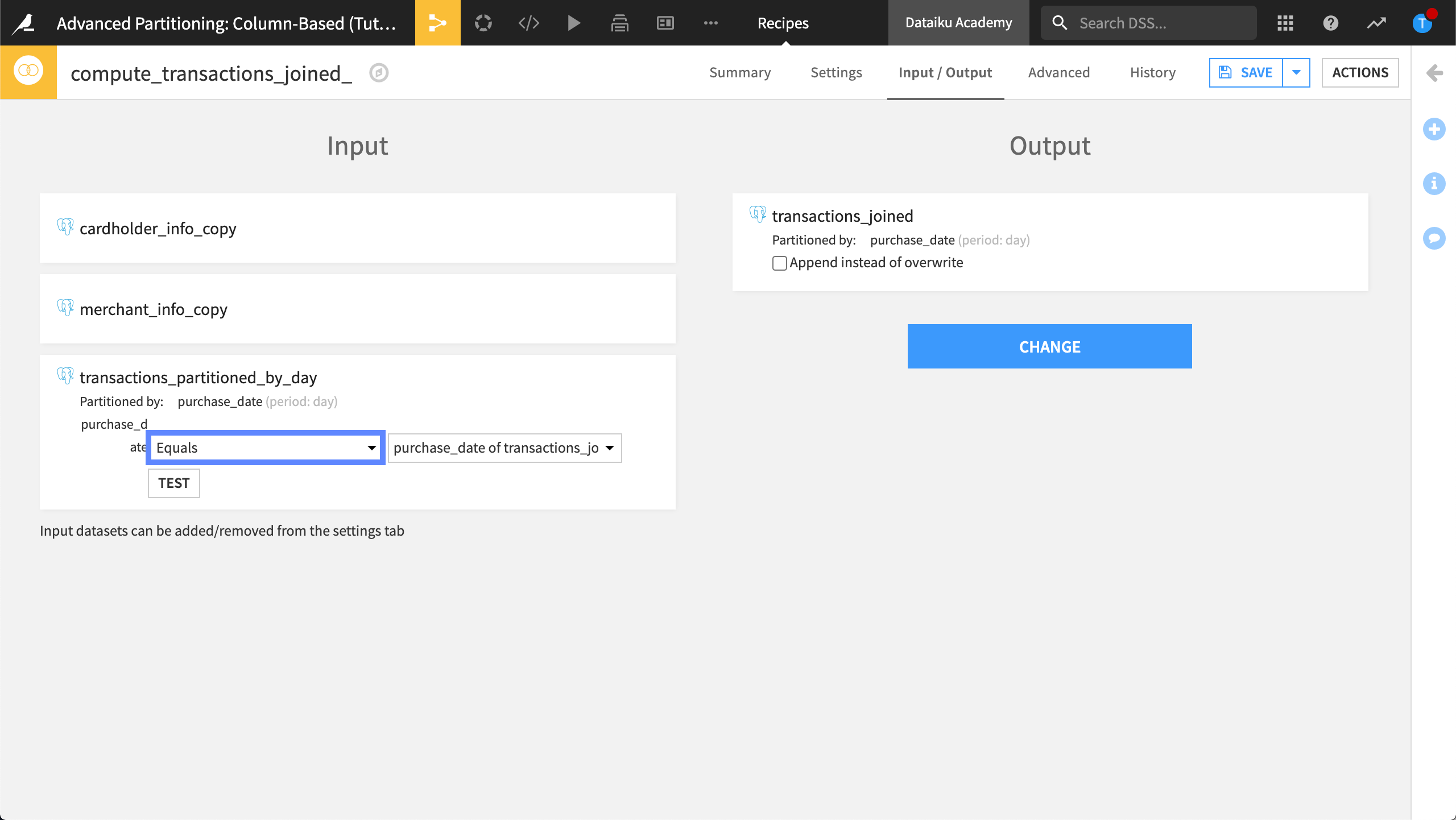
Open the Join recipe and view the Input / Output tab.
By default, Dataiku sets the partition mapping so that the output dataset is built, or partitioned, using all available partitions in the input dataset.
To optimize the Flow, we only want to target the specific partitions where we’re asking the recipe to perform computations.
In the partitions mapping, choose Equals as the partition dependency function type.
View the Settings tab.
Click the Recipe run options icon next the Run button, and select Specify explicitly.
Type the value,
2017-12-20,2017-12-21,2017-12-22,2017-12-23then click OK.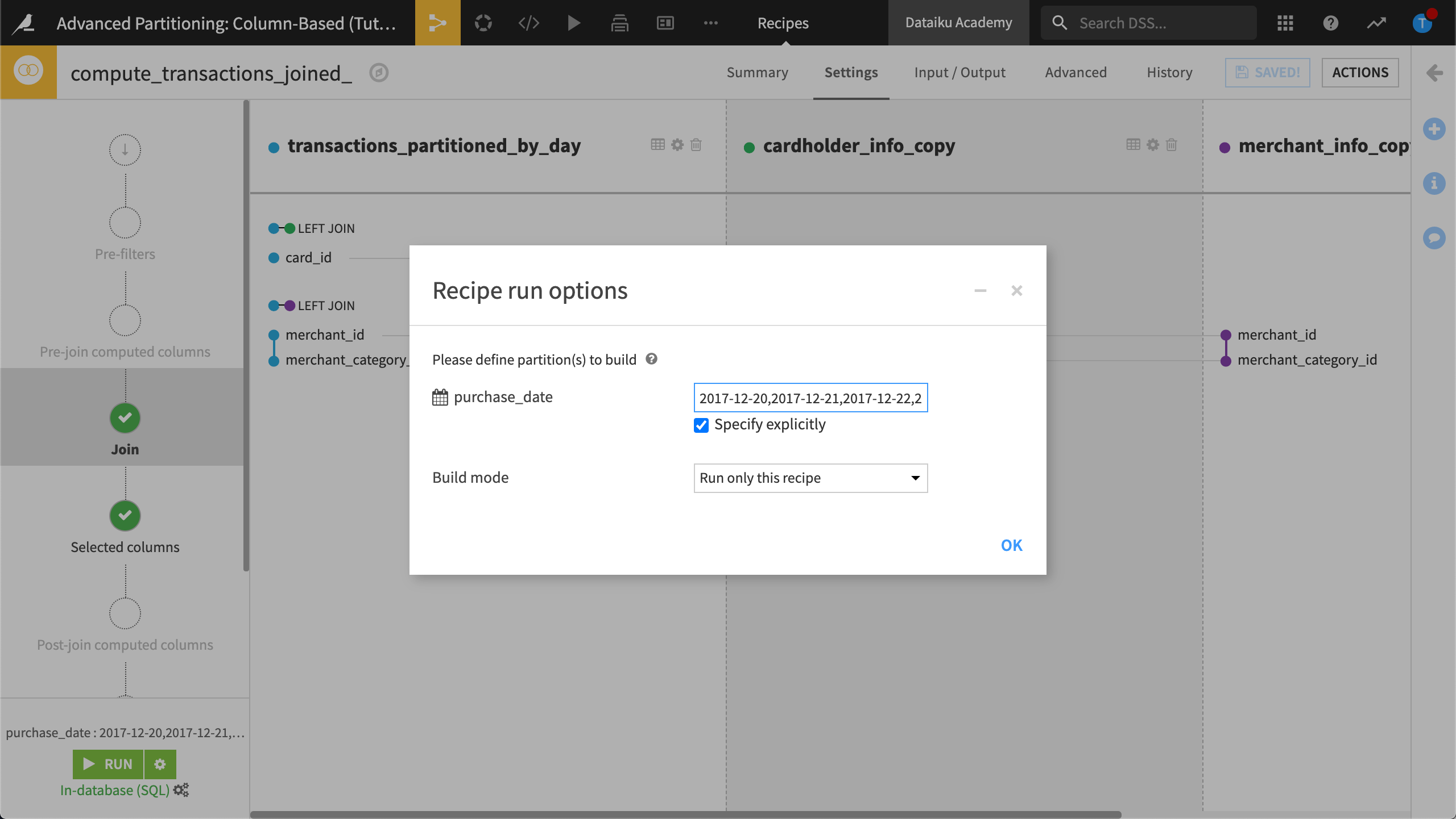
Without running the recipe, click Save and accept the schema change.
The recipe is now configured to compute the Join only on the rows belonging to the dates between
2017-12-20and2017-12-23.Don’t run the recipe yet.
Run a partitioned job#
Let’s run a partitioned job.
Return to the Flow.
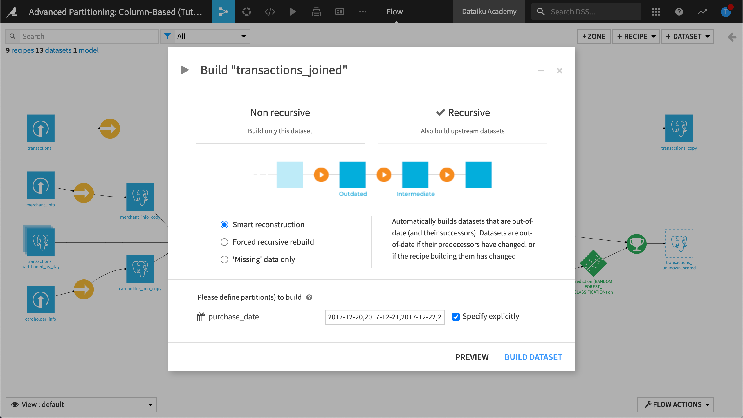
Right-click transactions_joined and select Build from the menu.
Choose a Recursive build.
Select Smart reconstruction.
Click Build Dataset.
View job and activity log#
Let’s view the job activity log to reveal how partitioned SQL jobs are managed.
View the most recent Job.
View the job Activities.
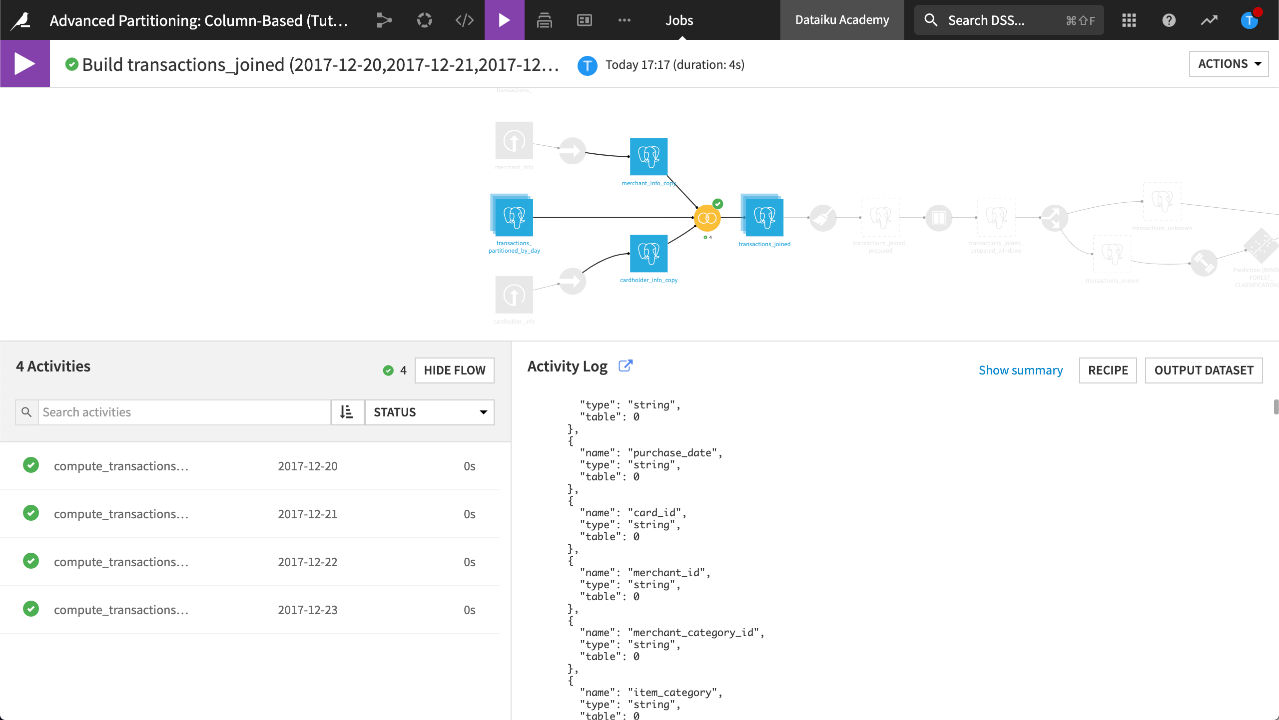
The Activity Log for the partition 2017-12-20 contains the following queries:
A query to delete rows from transactions_joined where the purchase date is
2017-12-20.A query to insert the rows belonging to the new partition into transactions_joined.
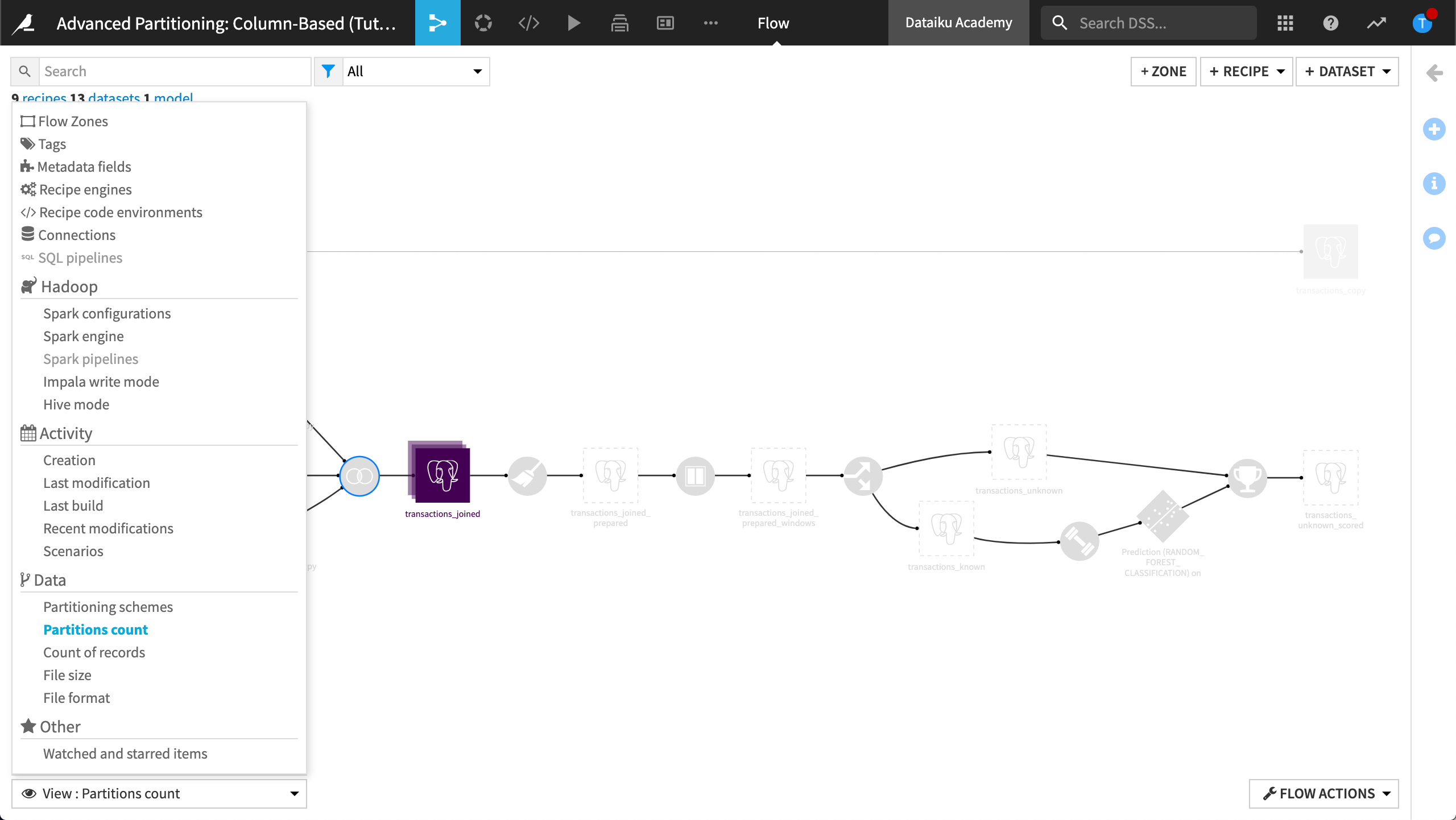
View partitions count in the Flow#
We can use a Flow view to discover whether the job is completed.
Return to the Flow.
From the Flow view, select to visualize the Partitions count.
The table, transactions_partitioned_by_day has zero partitions. To update this count:
Select transactions_partitioned_by_day.
In the right panel, click Update status (count of records, file size) to update the count.
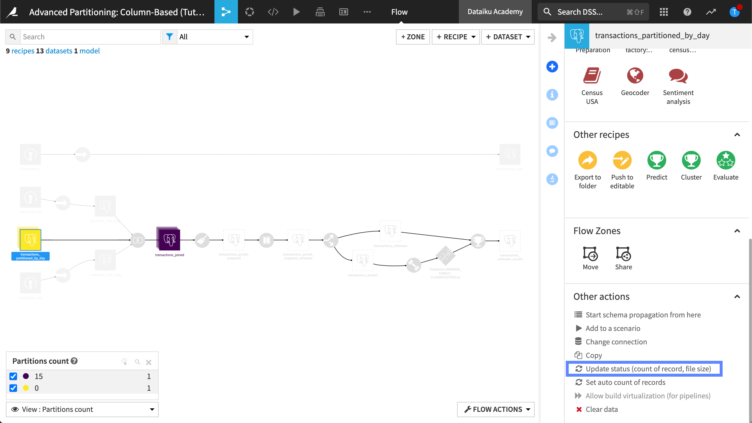
Wait while Dataiku updates the count of partitions, then refresh the page. The transactions_partitioned_by_day contains 15 time-based partitions.
Close the Partitions count view to restore the default view.
Build a non-partitioned output dataset#
We will now stop the partitioning of our purchase_date dimension and create a non-partitioned dataset. To do this, Dataiku uses a “partition collection” mechanism during runtime. This mechanism is triggered by the partition dependency function type, All available.
This process is referred to as partition collecting. Partition collecting can be thought of as the reverse of partition redispatching.
Open the Prepare recipe that’s used to create transactions_joined_prepared.
In the Input / Output tab, ensure the partition dependency function type is set to All available.
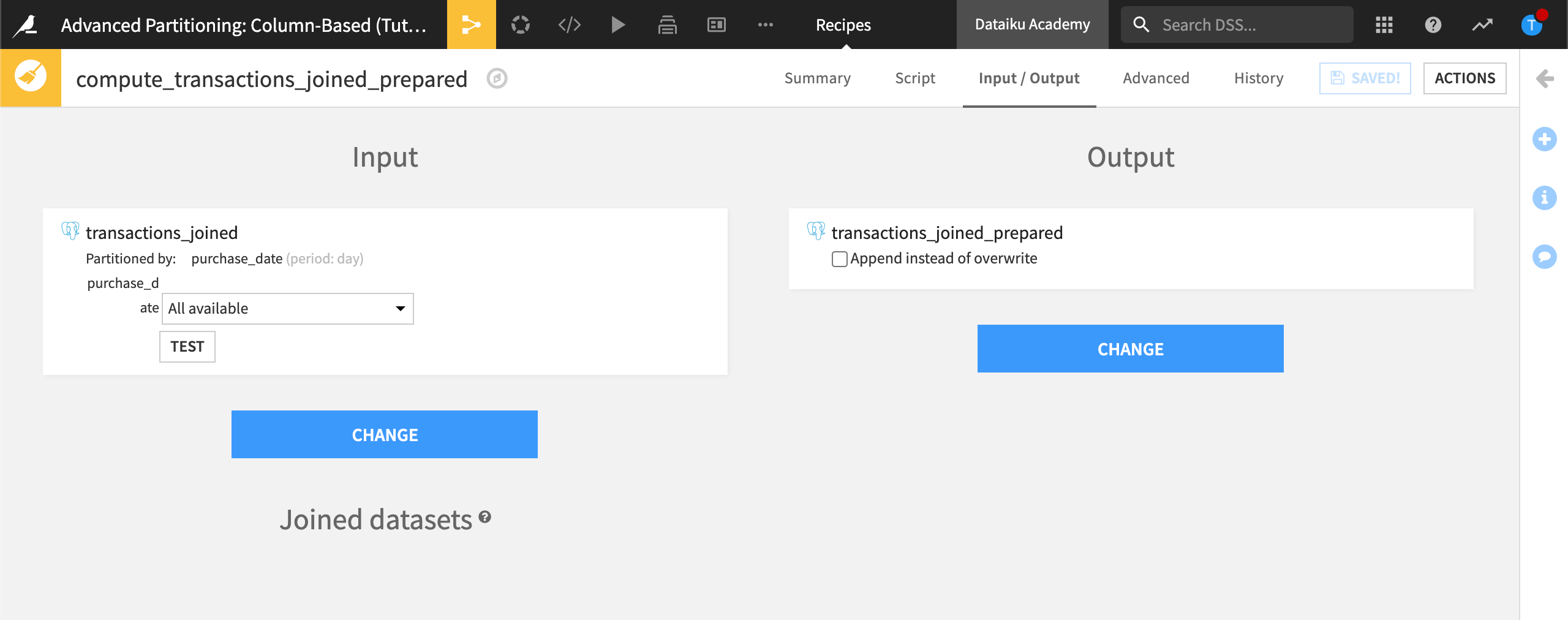
In the Script step, run the recipe.
All Available means all available input partitions will be processed when we run the recipe. The output dataset, transactions_joined_prepared, isn’t partitioned.
Build a discrete-based partitioned dataset#
Create a partitioned output#
Recall from the business objectives that we want to be able to predict whether a transaction is fraudulent based on the transaction subsector (for example insurance, travel, and gas) and the purchase date. This is discrete information.
To meet this objective, we need to partition the Flow with a discrete dimension. We want the input dataset, transactions_joined_prepared, of the Window recipe to be partitioned by merchant subsector.
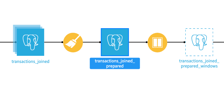
Create transactions_joined_prepared_windows#
The input dataset in our Window recipe, transactions_joined_prepared, isn’t partitioned. To partition this dataset, we can follow the same steps we followed when we created our time-based partitioned outputs. By creating a new, logical pointer, we can create a new dataset without duplicating the data.
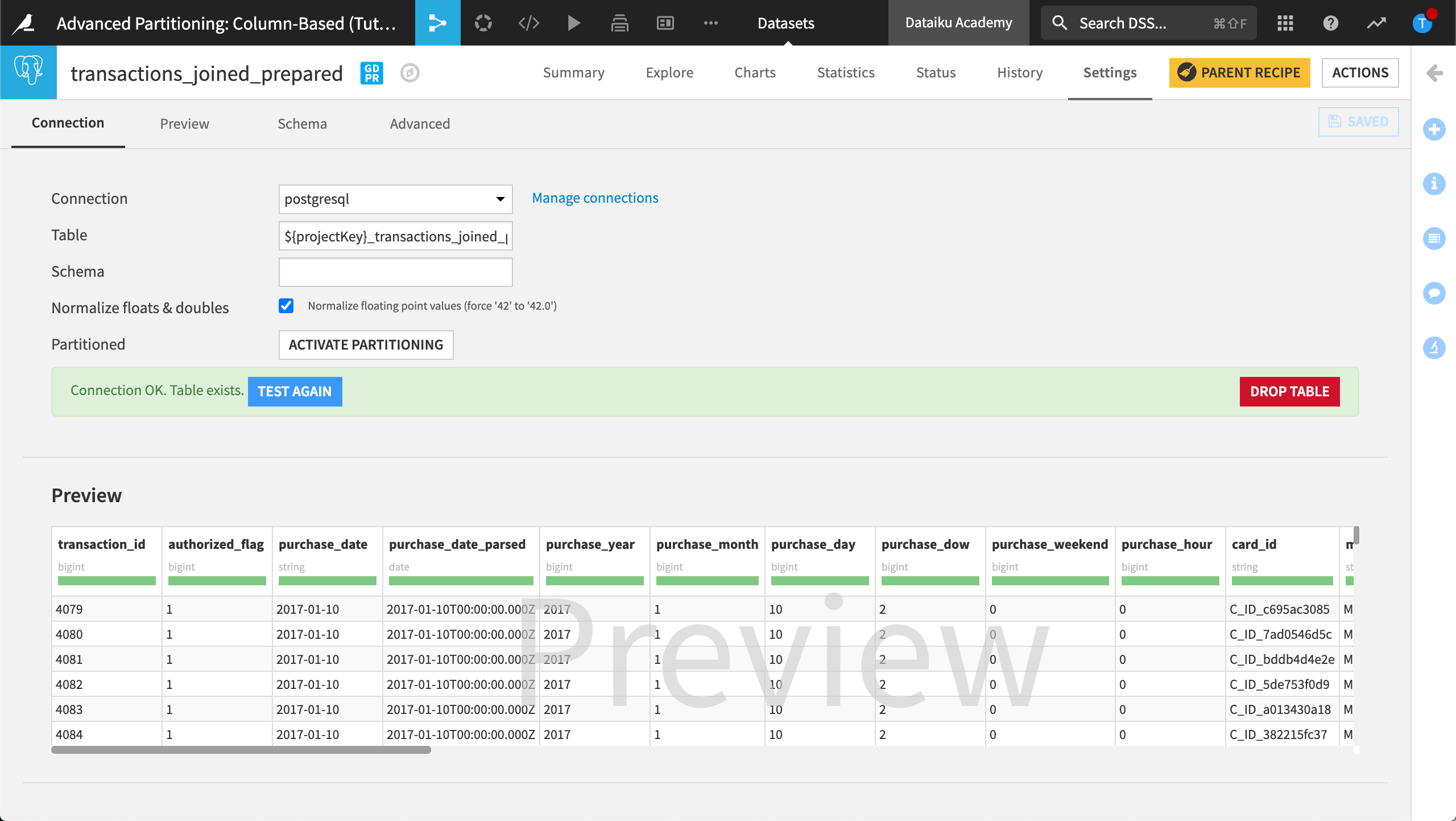
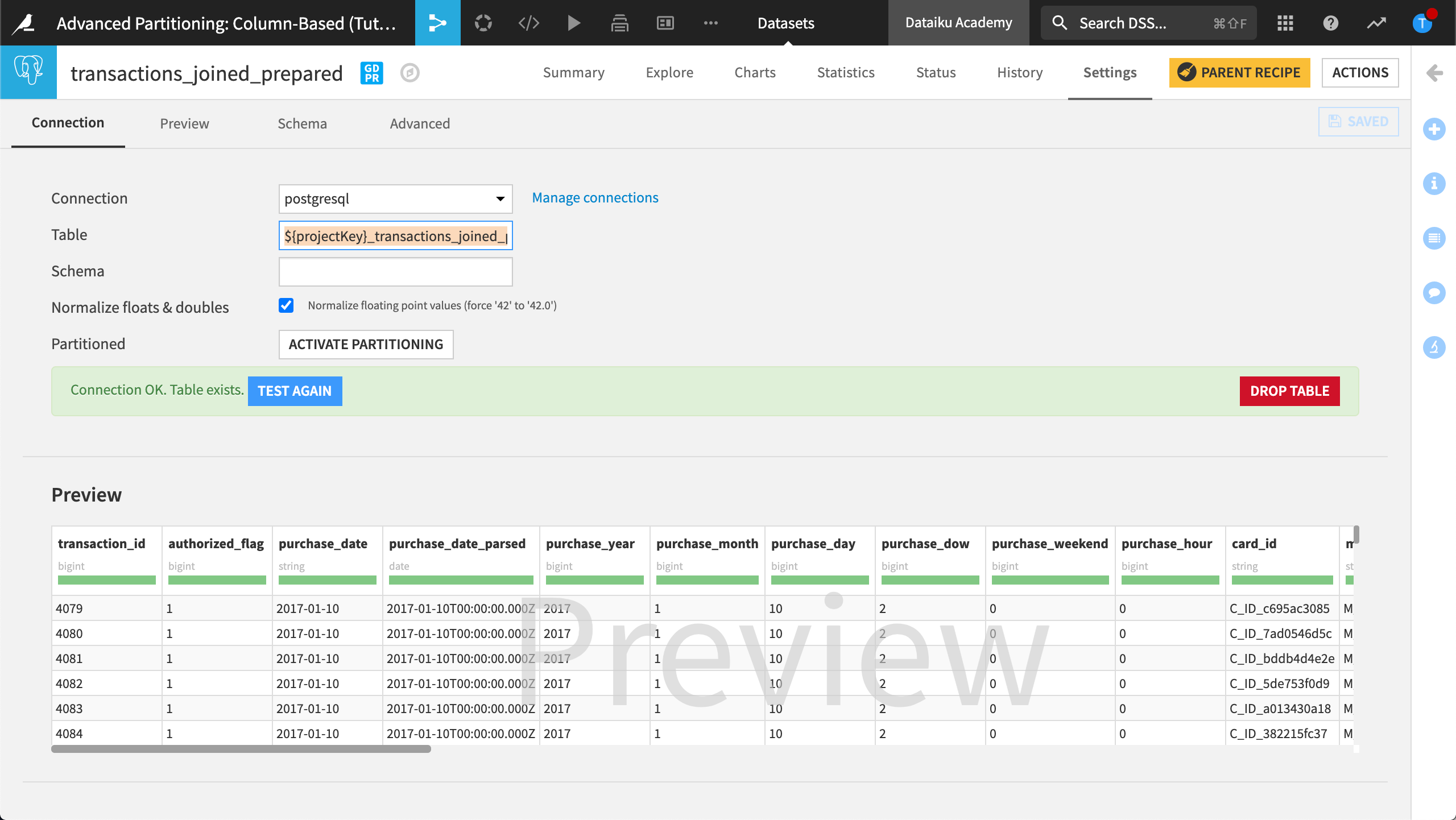
Open transactions_joined_prepared and view the Settings page.
Copy the contents of the Table and Schema fields and save the information for later.
Return to the Flow.
In the upper-right-hand corner, click +Dataset.
From the SQL databases menu, select your SQL connection.
Paste the information you saved from the Table and Schema fields.
Click Test Table.
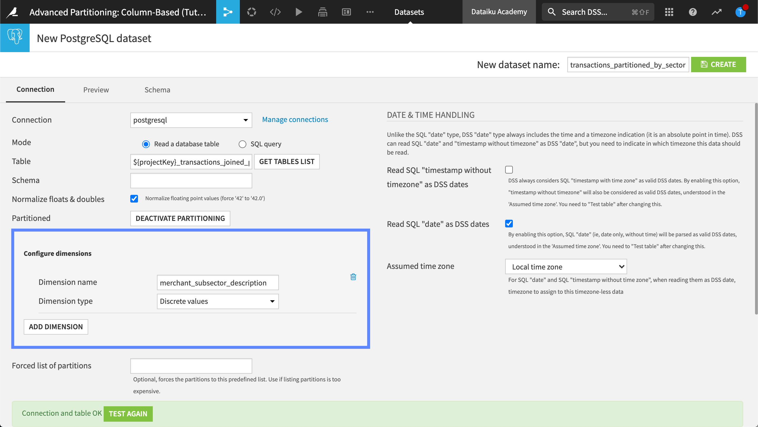
Next to Partitioned, click Activate Partitioning to enable discrete-based partitioning for this SQL dataset.
Name the dimension,
merchant_subsector_description.
Let’s create this dataset.
In the upper-right-hand corner, name the new dataset,
transactions_partitioned_by_sector.Click Create.
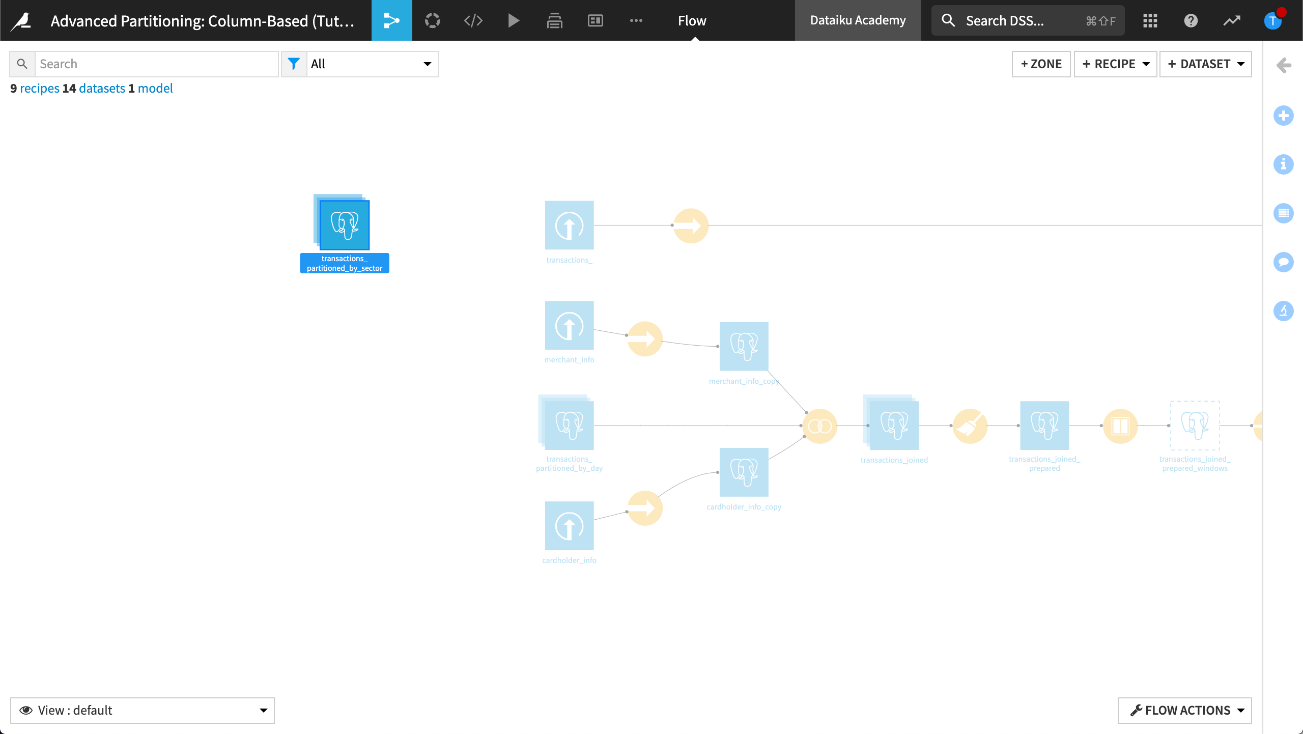
Our Flow now looks like this:
Configure the Window recipe#
Configure the Window recipe to change the input dataset from transactions_joined_prepared to transactions_partitioned_by_sector.
Open the Window recipe.
In the Input / Output tab, change the transactions_joined_prepared dataset to transactions_partitioned_by_sector.
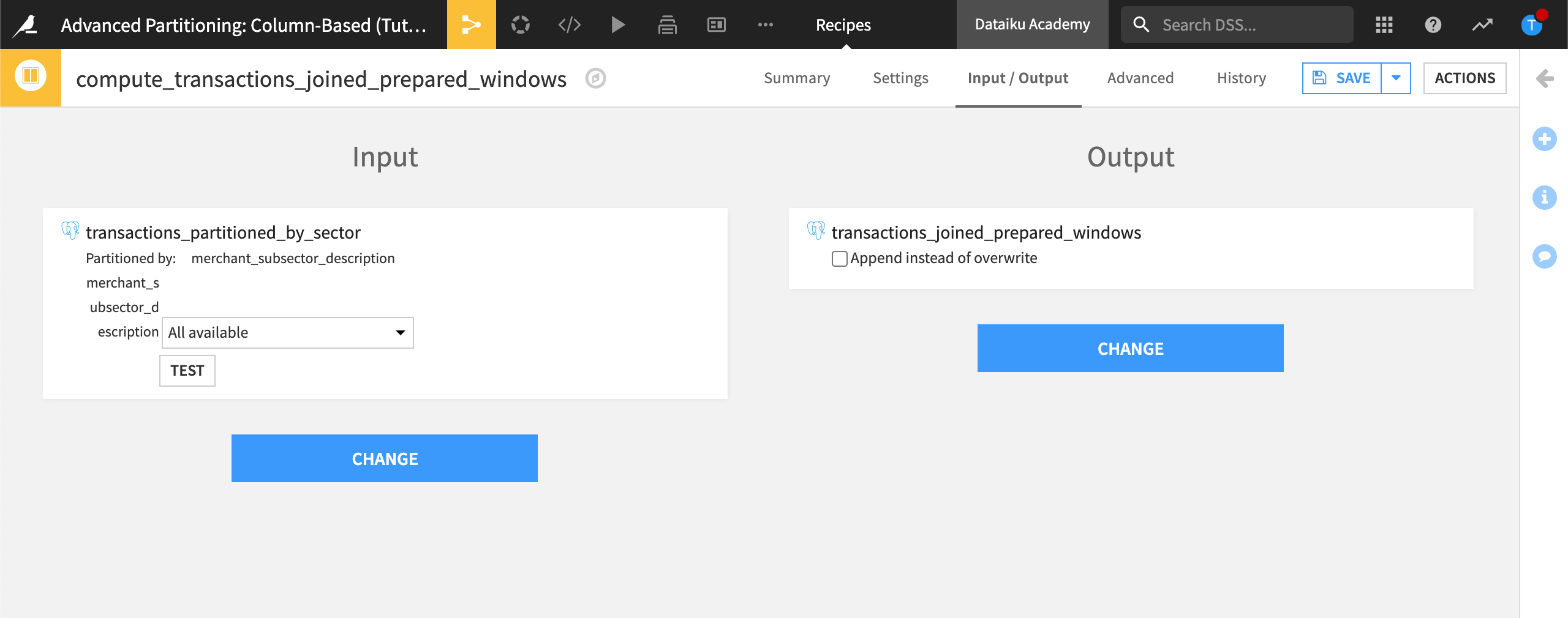
Save and run the recipe.
Return to the Flow.
Our Flow now looks like this:
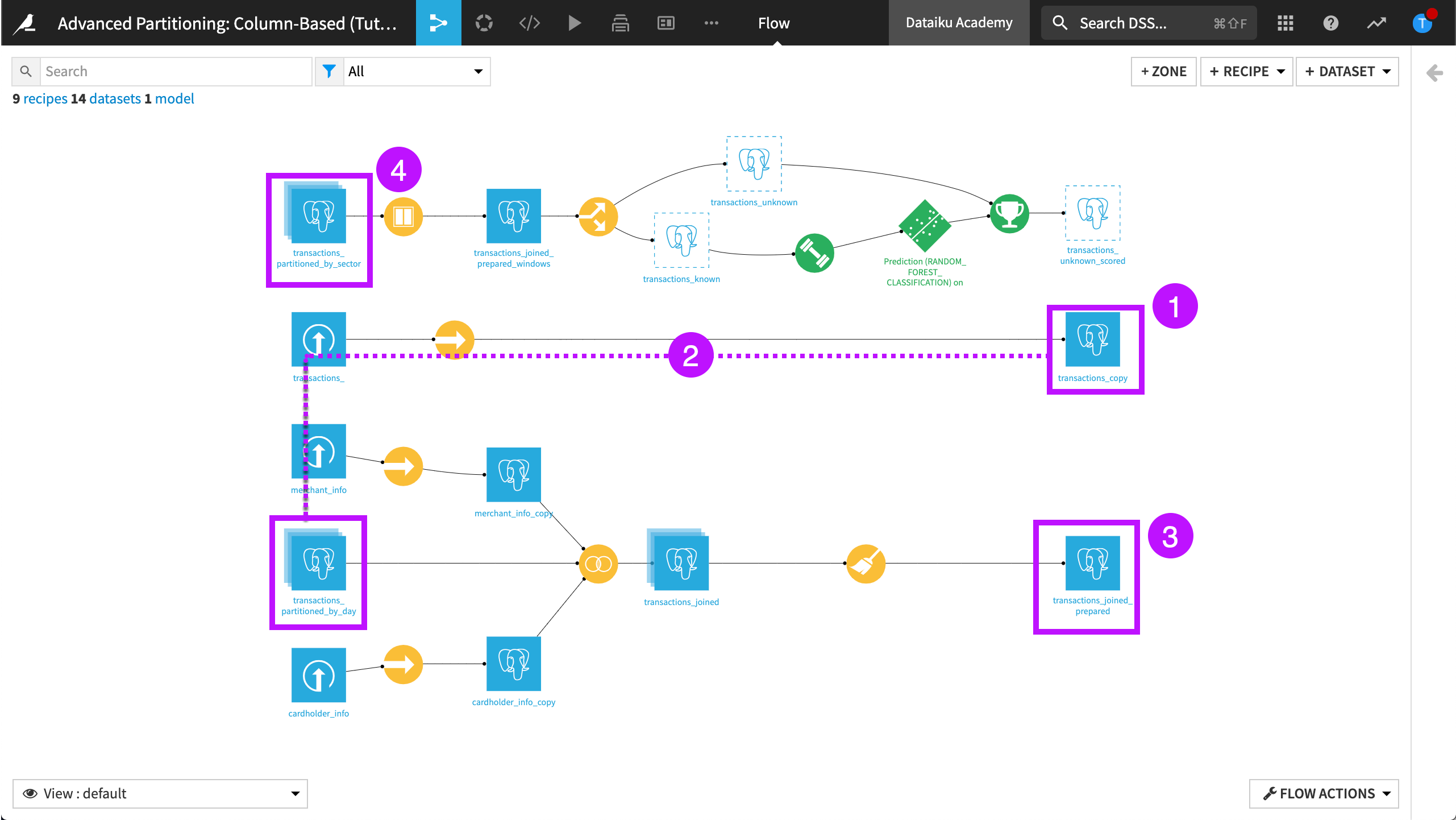
Recap#
Let’s look at this in more detail.
Data is written into the SQL table, ${projectKey}_transactions_copy. The dataset, transactions_copy is linked to this table.
A connection is created to the dataset, transactions_partitioned_by_day. This dataset is also linked to the table, ${projectKey}_transactions_copy, but it’s partitioned with the purchase_date dimension. Therefore, downstream datasets can also be partitioned by purchase_date.
Data is then written in the SQL table, ${projectKey}_transactions_joined_prepared. The dataset, transactions_joined_prepared is linked to this table.
Finally, a connection is created to the dataset, transactions_partitioned_by_sector. This dataset is also linked to the table ${projectKey}_transactions_joined_prepared, but it’s partitioned by merchant subsector. Therefore, downstream datasets can also be partitioned by merchant subsector.
View partitions count in the Flow#
Return to the Flow.
From the Flow view, select to visualize the Partitions count.
Select transactions_partitioned_by_sector and update the count of records.
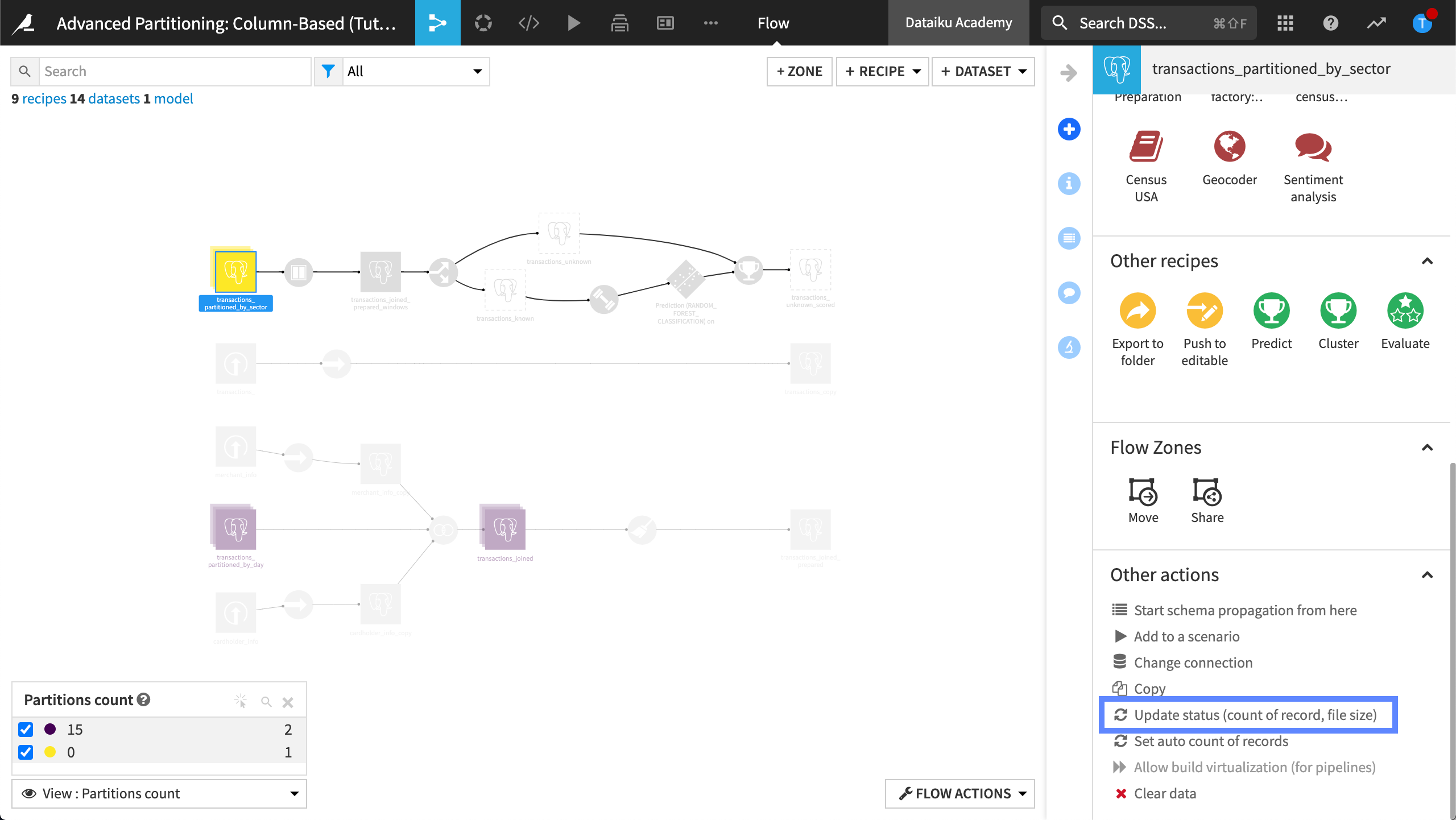
Wait while Dataiku updates the count of partitions, then refresh the page.
The transactions_partitioned_by_sector dataset contains 9 partitions.
Close the Flow view.
Propagate the discrete partitioning through the Flow#
Now you can apply what you’ve learned to propagate the discrete partitioning through the Flow. To do this, follow the same process you used to propagate the time-based partitioning through the Flow.
Run the Split recipe.
Partition the following datasets by the merchant_subsector_description dimension:
Partition transactions_joined_prepared_windows
Partition transactions_known
Partition transactions_unknown
Partition transactions_unknown_scored
Congratulations! You have completed the tutorial.
Next steps#
Visit the course, Partitioned Models, to learn more about training a machine learning model on the partitions of a dataset.