
Going deeper into churn modeling#
In the previous section, we generated a test set containing the target variable, we should then be able to evaluate our model on this dataset.
Doing so will give us a better approximation of the real model performance, since it takes time into account. We used previously the default random 80% (train) / 20% (test) split, but this assumes that our Flow and model are time-independent, an assumption clearly violated in our construction.
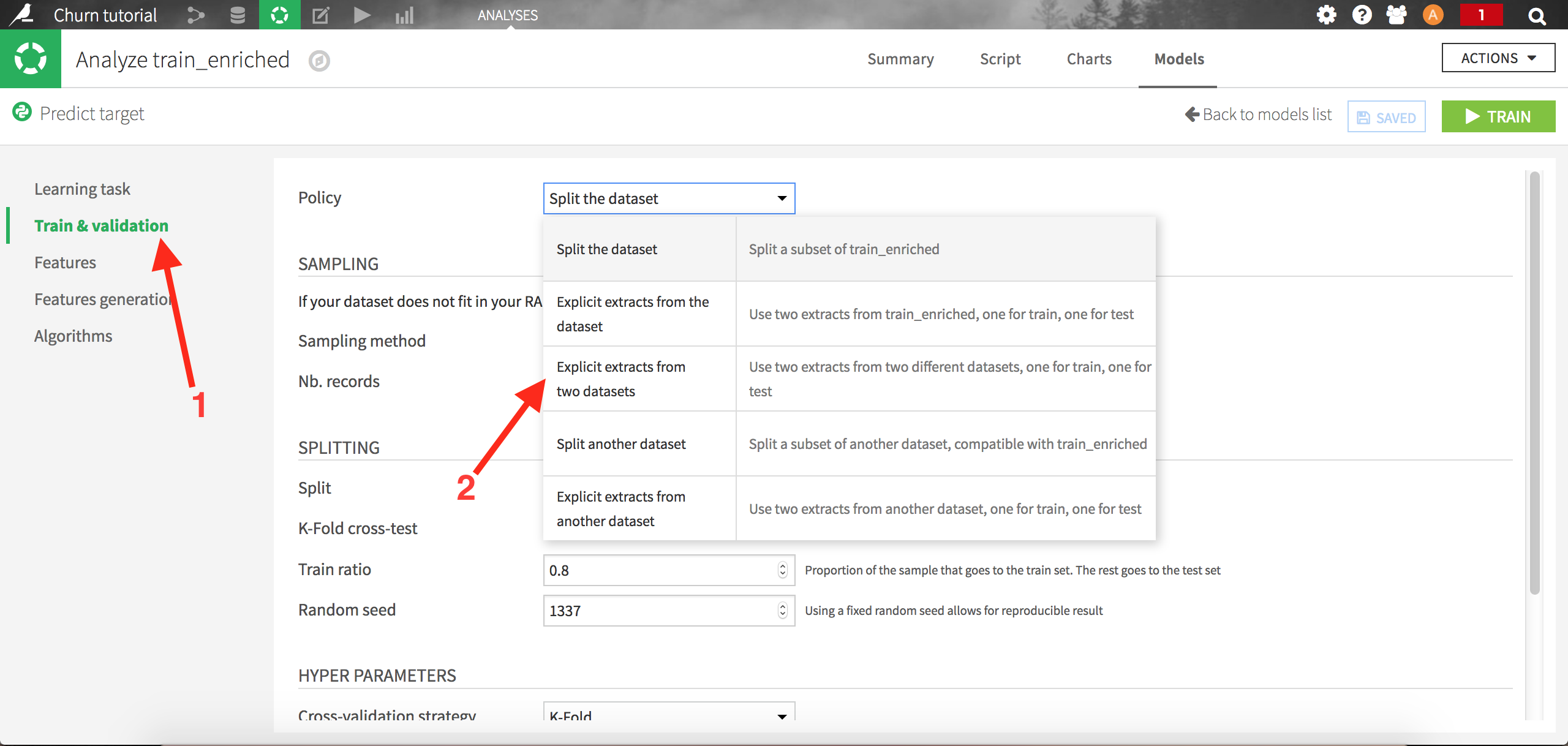
Let’s go back to our model, and go to the settings screens. We’re going to change the Train & validation policy. Let’s choose “Explicit extracts from two datasets”:
Choose test_enriched as the Test Set and save. Dataiku will now train the models on the train set, and evaluate it using an auxiliary test set (test_enriched):
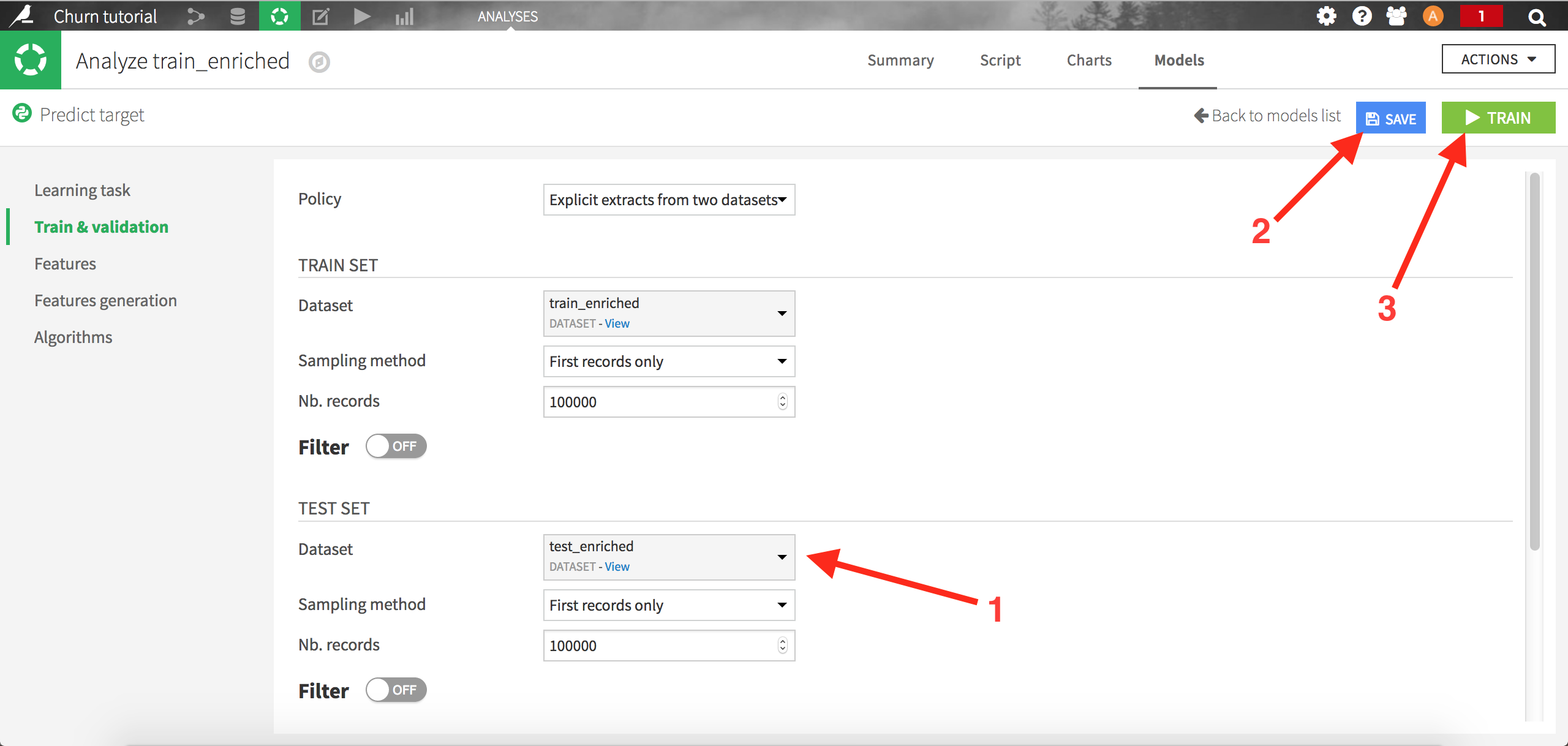
Click on “train” to start the calculations. The summary model list should now be updated with new runs:
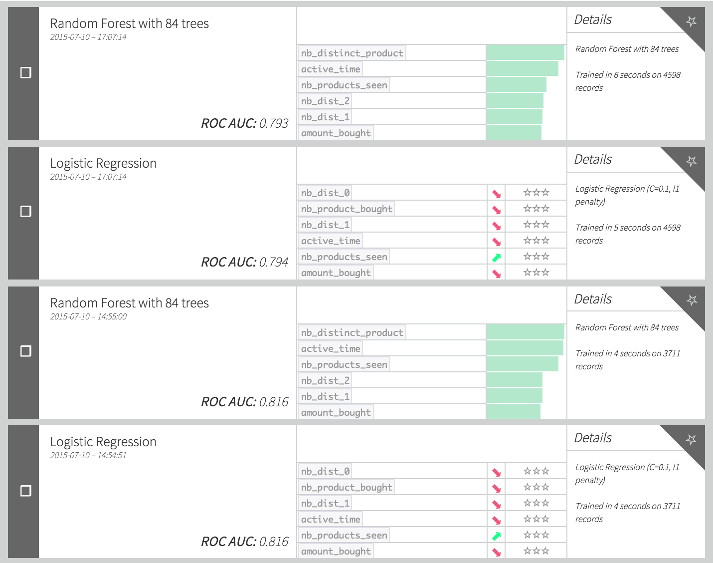
Note that the performance (here measured via the AUC) decreased a lot, even though we’re using more data (because there is no train split, we have 1.25 times more data in our train set). The reason of this decrease is the combination of 2 factors:
Things inherently change with time. The patterns observed in our train set may have changed in the test set, since this one uses fresher data. Even though this effect can be rather small, it will however always exist when dealing with time dependent data (and train/test split strategy), and this is something that needs to be taken into account when creating such models.
Our features are poorly designed, since we created them using the whole history of data. The amount of data available to build the features increases over time: here the test set would rely on a much longer history than the train set (because the train set uses “older” data), so our features distributions would differ a lot between the train set and the test set.
This issue can be solved by designing smarter features, like count of product seen in the past “k” weeks from the reference date, or by creating ratios such as the total amount spent divided by total duration of user activity. We can then transform the code used to generate the train_enriched dataset this way:
SELECT
  -- Basic features
  basic.*,
  -- "Trend" features
  one.nb_products_seen::numeric / basic.nb_products_seen AS rap_nb_products_seen ,
  one.nb_distinct_product::numeric / basic.nb_distinct_product AS rap_nb_distinct_product,
  one.nb_dist_0::numeric / basic.nb_dist_0 AS rap_nb_nb_dist_0 ,
  one.nb_dist_1::numeric / basic.nb_dist_1 AS rap_nb_dist_1 ,
  one.nb_dist_2::numeric / basic.nb_dist_2 AS rap_nb_dist_2 ,
  one.nb_seller::numeric / basic.nb_seller AS rap_nb_seller ,
  one.amount_bought::numeric / basic.amount_bought AS rap_amount_bought ,
  one.nb_product_bought::numeric / basic.nb_product_bought AS rap_nb_product_bought ,
  -- global features
  glob.amount_bought / active_time AS amount_per_time ,
  glob.nb_product_bought::numeric / active_time AS nb_per_time ,
  glob.amount_bought AS glo_bought ,
  glob.nb_product_bought AS glo_nb_bought ,
  -- target
  target
FROM
  train

  LEFT JOIN (
    SELECT
      user_id,
      COUNT(product_id) AS nb_products_seen,
      COUNT(distinct product_id) AS nb_distinct_product,
      COUNT(distinct category_id_0) AS nb_dist_0,
      COUNT(distinct category_id_1) AS nb_dist_1,
      COUNT(distinct category_id_2) AS nb_dist_2,
      COUNT(distinct seller_id) AS nb_seller ,
      SUM(price::numeric * (event_type = 'buy_order')::int ) AS amount_bought,
      SUM((event_type = 'buy_order')::int ) AS nb_product_bought
    FROM
      events_complete
    WHERE
          event_timestamp <  TIMESTAMP '${churn_test_date}'
                           - INTERVAL '${churn_duration} months'
      AND event_timestamp >= TIMESTAMP '${churn_test_date}'
                           - 2 * INTERVAL '${churn_duration} months'
    GROUP BY
      user_id
  ) basic ON train.user_id = basic.user_id

  LEFT JOIN (
    SELECT
      user_id,
      COUNT(product_id) AS nb_products_seen,
      COUNT(distinct product_id) AS nb_distinct_product,
      COUNT(distinct category_id_0) AS nb_dist_0,
      COUNT(distinct category_id_1) AS nb_dist_1,
      COUNT(distinct category_id_2) AS nb_dist_2,
      COUNT(distinct seller_id) AS nb_seller,
      SUM(price::numeric * (event_type = 'buy_order')::int ) AS amount_bought,
      SUM((event_type = 'buy_order')::int ) AS nb_product_bought
    FROM
      events_complete
    WHERE
         event_timestamp <  TIMESTAMP '${churn_test_date}'
                          - INTERVAL '${churn_duration} months'
     AND event_timestamp >= TIMESTAMP '${churn_test_date}'
                          - INTERVAL '${churn_duration} months'
                          - INTERVAL '1 months'
    GROUP BY
      user_id
) one ON train.user_id = one.user_id

LEFT JOIN (
  SELECT
    user_id,
    SUM(price::numeric * (event_type = 'buy_order')::int ) AS amount_bought,
    SUM((event_type = 'buy_order')::int ) AS nb_product_bought,
    EXTRACT(
     EPOCH FROM (
        TIMESTAMP '${churn_test_date}'
      - INTERVAL '${churn_duration} months'
      - MIN(event_timestamp)
     )
    ) / (3600*24) AS active_time
  FROM
    events_complete
  WHERE
    event_timestamp < TIMESTAMP '${churn_test_date}'
                    - INTERVAL '${churn_duration} months'
  GROUP BY
    user_id
) glob ON train.user_id = glob.user_id
This SQL recipe looks rather cumbersome, but if we look at it more in details, we see that we generated three kinds of variables:
“basic” features, which are the exact same counts and sums as in the previous section, except that they’re now based only on the previous rolling month. This way, our variables are less dependent on time.
“trend” variables, which are the ratio between the features calculated on one rolling week, and those calculated on one rolling month. With these variables, we intend to capture if the consumer has been recently increasing or decreasing its activity.
“global” features, which capture the information on the whole customer life. These variables are rescaled by the total lifetime of the customer so as to be less correlated with time.
By adapting in the same way the test_enriched dataset (modifying table names and dates in the query), you should be able to retrain your model, and have performances similar to this:
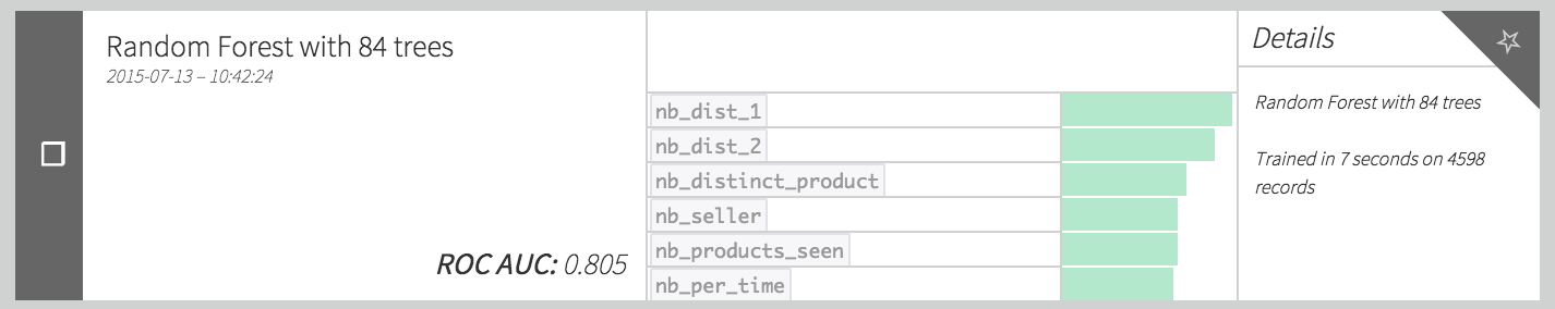
We managed to improve our performance by more than 0.01 point of AUC, doing some basic feature engineering.