Quick Start | Dataiku for machine learning#

Get started#

Recent advancements in generative AI have made it easy to apply for jobs. But be careful! Scammers have also been known to create fake job applications in the hopes of stealing personal information. Let’s see if you—with Dataiku’s help—can spot a real job posting from a fake one!

Objectives#

In this quick start, you’ll:

Use a visual recipe to divide data into training and testing sets.
Train prediction models for a binary classification task.
Iterate on the design of a model training session.
Apply a chosen model to new data.

Create an account#

To follow along with the steps in this tutorial, you need access to a 12.0+ Dataiku instance. If you don’t already have access, you can get started in one of two ways:

Start a 14 day free trial. See How-to | Begin a free trial from Dataiku for help if needed.
Install the free edition locally for your operating system.

Open Dataiku#

The first step is getting to the homepage of your Dataiku Design node.

Go to the Launchpad.
Click Open Instance in the Design node tile of the Overview panel once your instance has powered up.

Important

If using a self-managed version of Dataiku, including the locally downloaded free edition on Mac or Windows, open the Dataiku Design node directly in your browser.

Once you are on the Design node homepage, you can create the tutorial project.

Create the project#

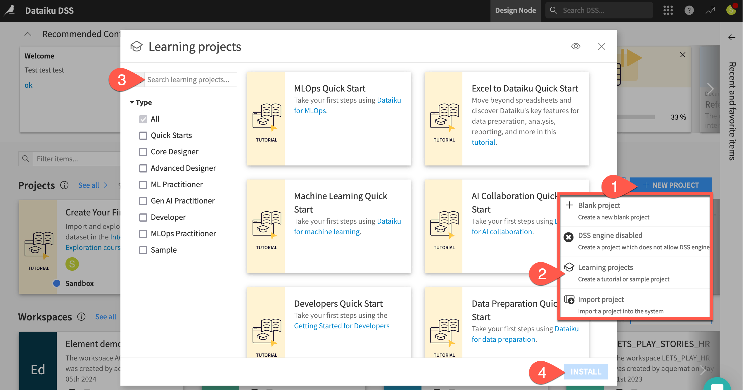
From the Dataiku Design homepage, click + New Project.
Select Learning projects.
Search for and select Machine Learning Quick Start.
If needed, change the folder into which the project will be installed, and click Install.
From the project homepage, click Go to Flow (or type g + f).

From the Dataiku Design homepage, click + New Project.
Select DSS tutorials.
Filter by Quick Starts.
Select Machine Learning Quick Start.
From the project homepage, click Go to Flow (or type g + f).

Note

You can also download the starter project from this website and import it as a zip file.

Review the Flow#

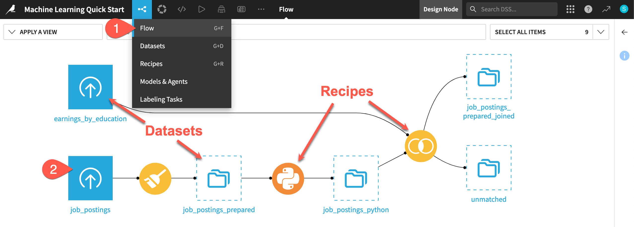
One of the first concepts a user needs to understand about Dataiku is the Flow. The Flow is the visual representation of how datasets, recipes (steps for data transformation), and models work together to move data through an analytics pipeline.

See the Flow’s visual grammar#

Dataiku has its own visual grammar to organize AI, machine learning, and analytics projects in a collaborative way.

Shape	Item	Icon
	Dataset	The icon on the square represents the dataset’s storage location, such as Amazon S3, Snowflake, PostgreSQL, etc.
	Recipe	The icon on the circle represents the type of data transformation, such as a broom for a Prepare recipe or coiled snakes for a Python recipe.
	Model	The icon on the diamond represents the type of modeling task, such as prediction, clustering, time series forecasting, etc.

Tip

In addition to shape, color has meaning too.

Datasets are blue. Those shared from other projects are black.
Visual recipes are yellow. Code recipes are orange. LLM recipes are pink. Plugin recipes are red.
Machine learning elements are green.

Take a look now!

If not already there, from the () menu in the top navigation bar, select the Flow (or use the keyboard shortcut g + f).
Double click on the job_postings dataset to open it.

Tip

There are many other keyboard shortcuts beyond g + f. Type ? to pull up a menu or see the Accessibility page in the reference documentation.

Analyze the data#

This project begins from a labeled dataset named job_postings composed of 95% real and 5% fake job postings. For the column fraudulent, values of 0 and 1 represent real and fake job postings, respectively. Your task will be to build a prediction model capable of classifying a job posting as real or fake.

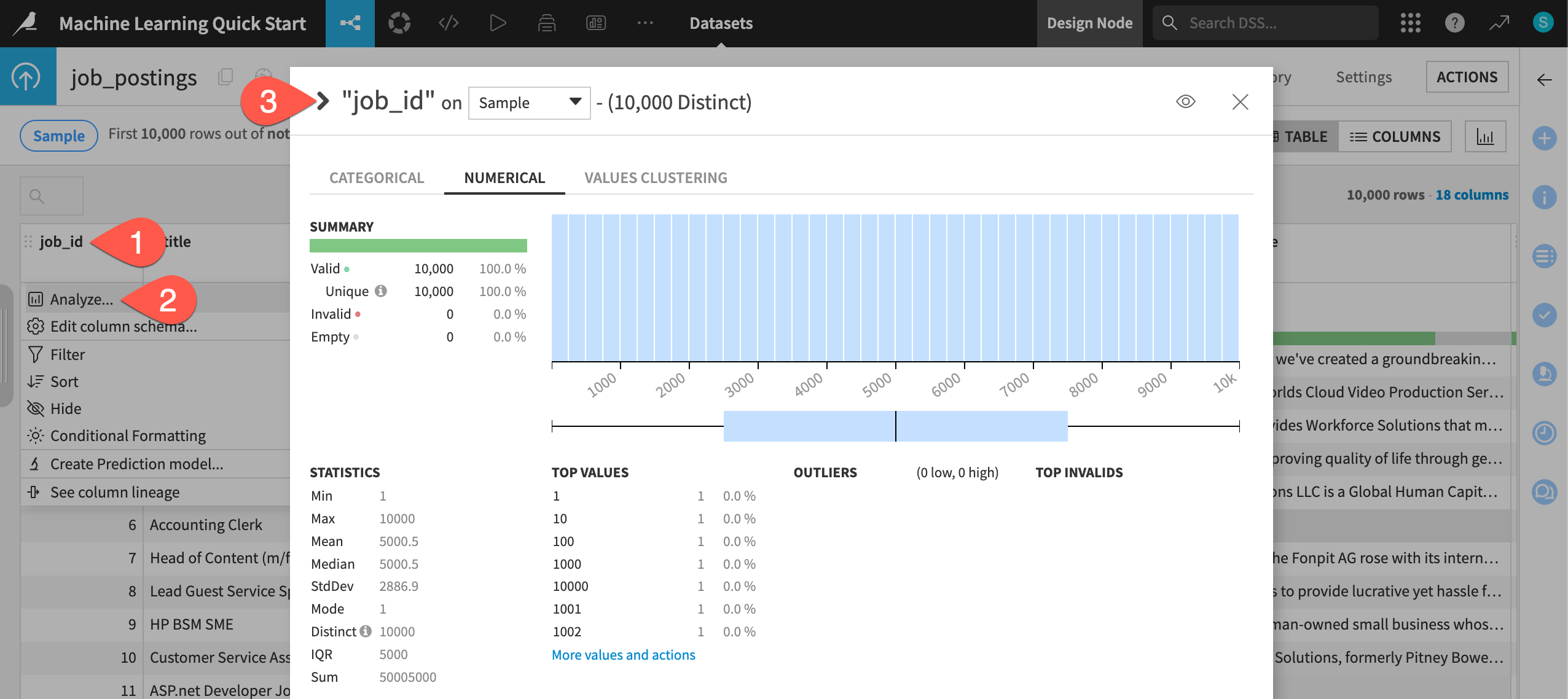
Take a quick look at the data.

Click on the header of the first column job_id to open a menu of options.
Select Analyze.
Use the arrows at the top left of the dialog to cycle through presentations of each column summary, including the target variable fraudulent column.

Build the Flow#

Unlike the initial uploaded datasets, the downstream datasets appear as outlines. This is because you haven’t built them yet. However, this isn’t a problem because the Flow contains the recipes required to create these outputs at any time.

Navigate back to the Flow (g + f).
Click to open the Flow Actions menu.
Click Build all.
Click Build to run the recipes necessary to create the items furthest downstream.
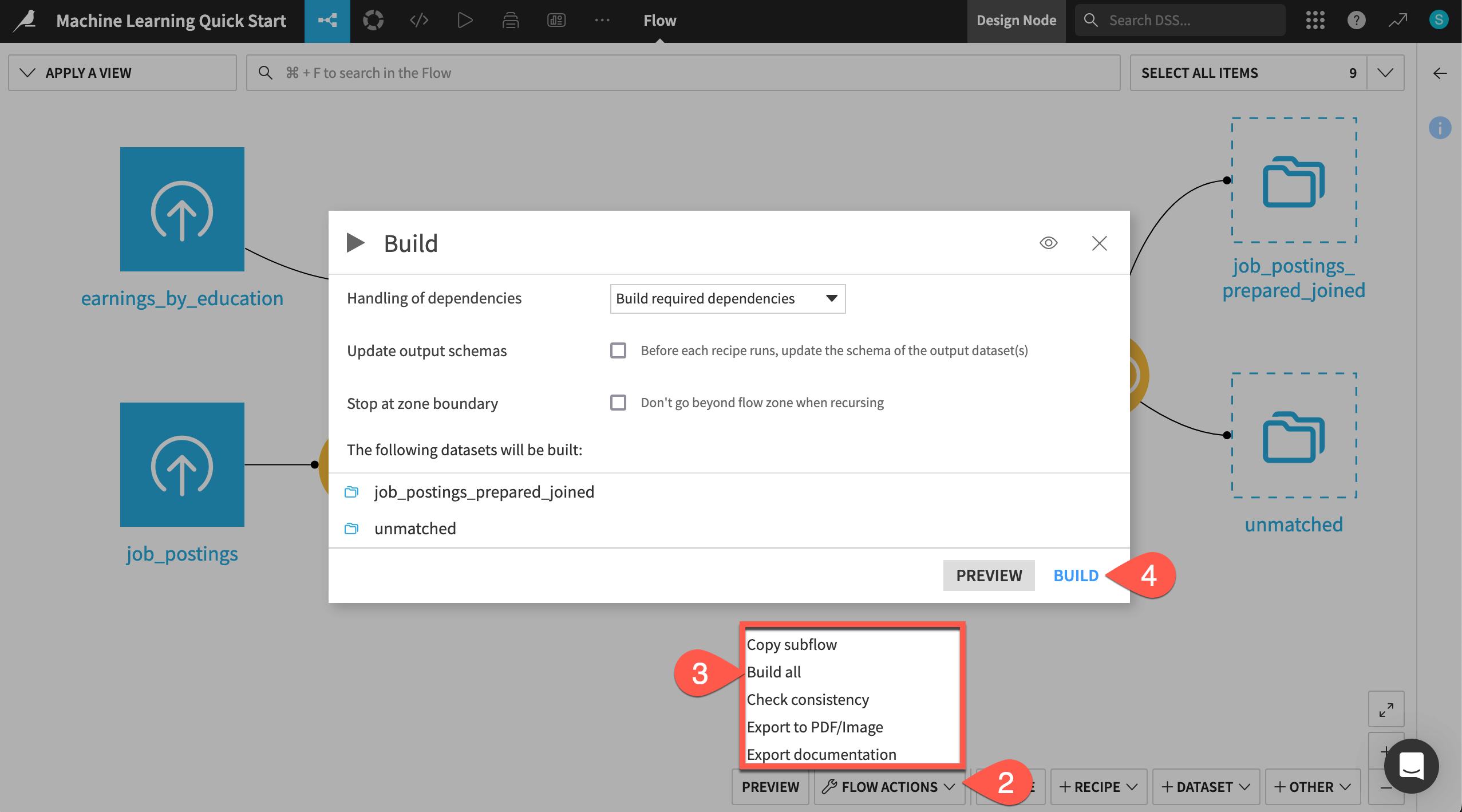
When the job completes, refresh the page to see the built Flow.

Split data into training and testing sets#

One advantage of an end-to-end platform like Dataiku is that you can do data preparation in the same tool as machine learning. For example, before building a model, you may wish to create a holdout set.

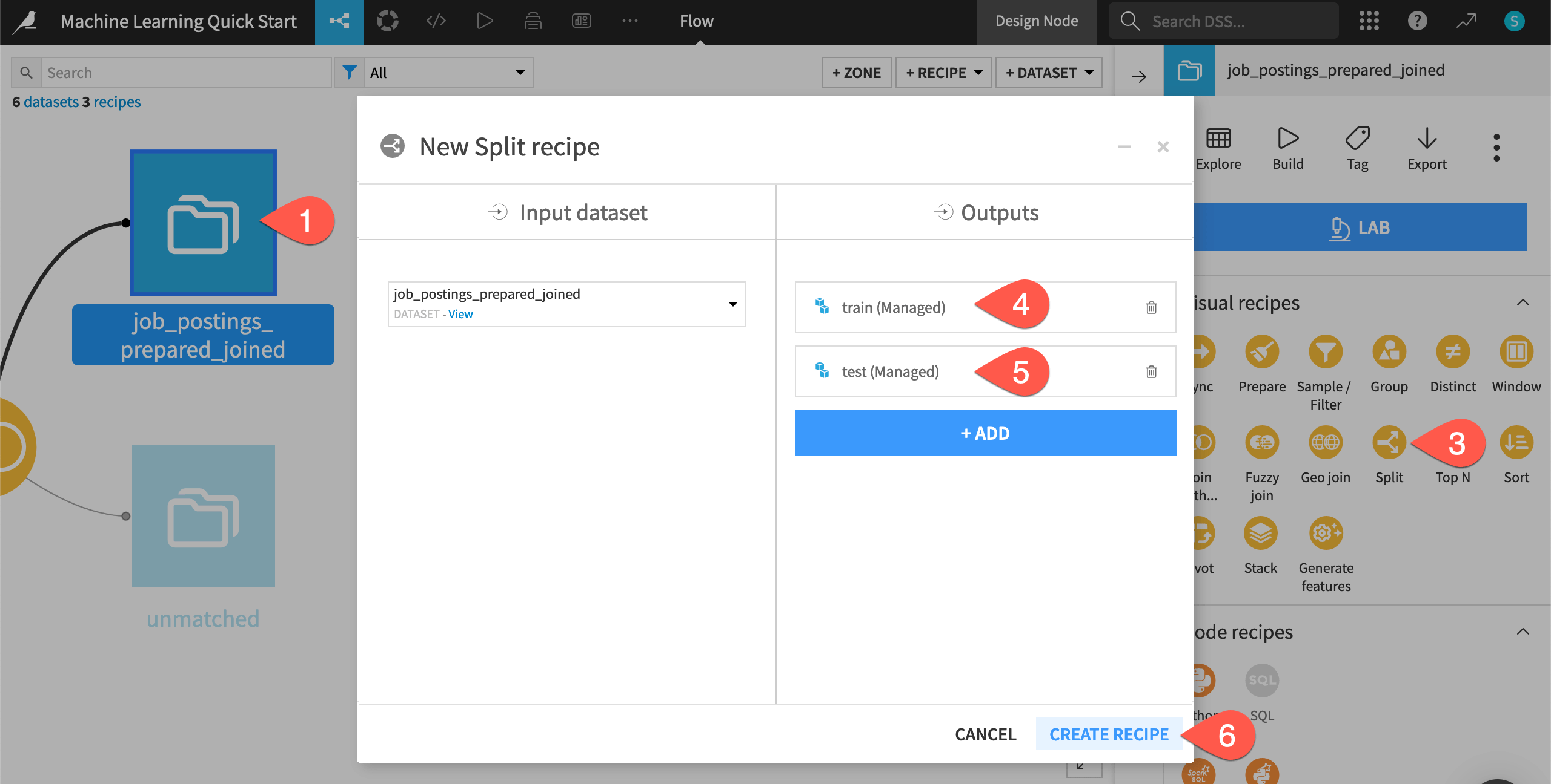
Let’s do this with a visual recipe.

From the Flow, click once to select the job_postings_prepared_joined dataset.
Open the Actions () tab of the right panel.
Select Split from the menu of visual recipes.
Click + Add; name the output train; and click Create Dataset.
Click + Add again; name the second output test; and click Create Dataset.
Once you have defined both output datasets, click Create Recipe.

Define a Split method#

The Split recipe allows for division of the input dataset into some number of output datasets in different ways. Possible splitting methods include mapping values of a column, defining filters, or as you’ll see here, randomly:

On the Splitting step of the recipe, select Randomly dispatch data as the splitting method.
Set the ratio of 80 % to the train dataset, and the remaining 20% to the test dataset.
Click the Run (or type @ + r + u + n) to build these two output datasets.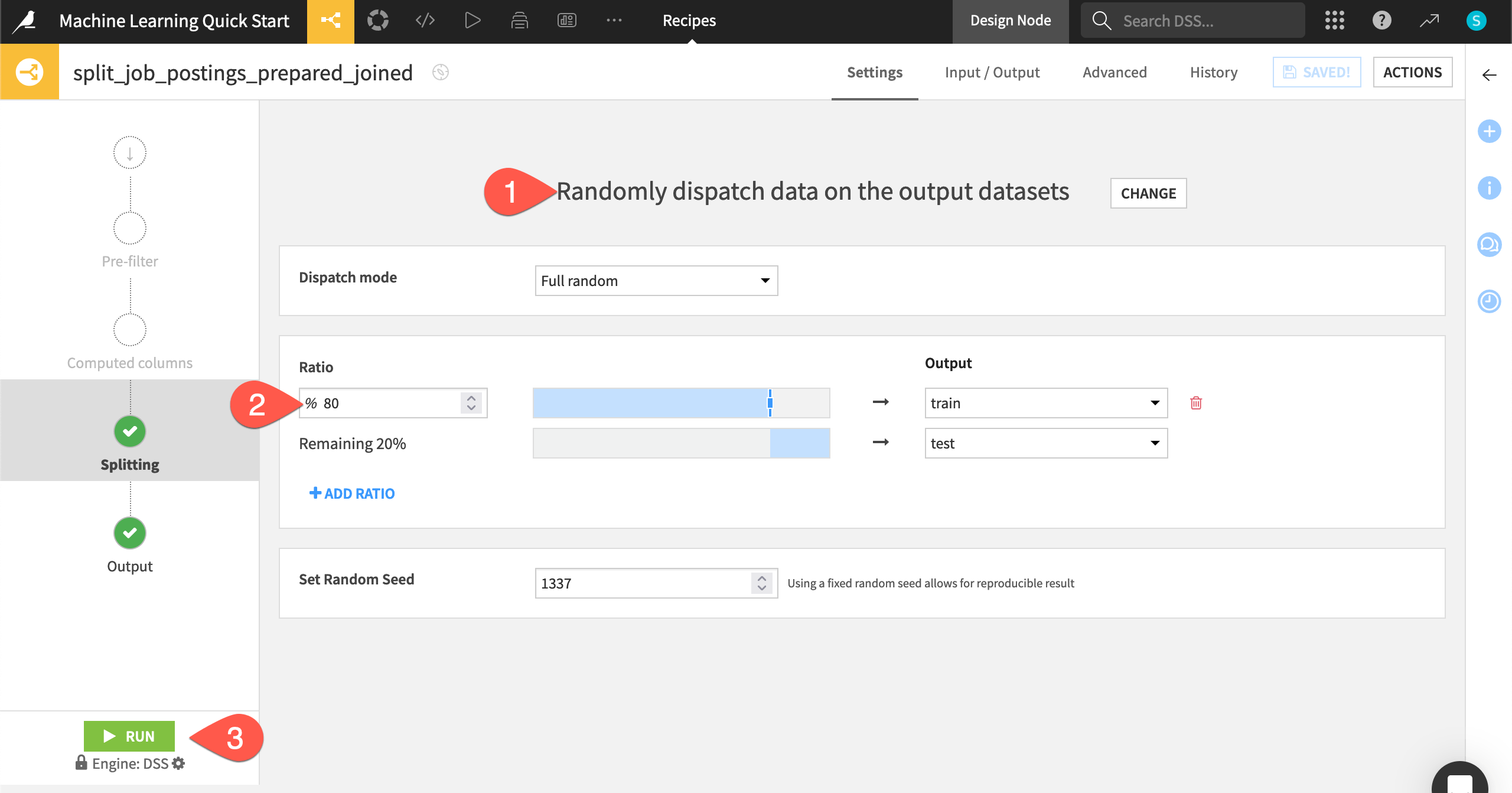
When the job finishes, navigate back to the Flow (g + f) to see your progress.

Create a separate Flow zone#

Before you start training models, there’s one organizational step that will be helpful as your projects grow in complexity.

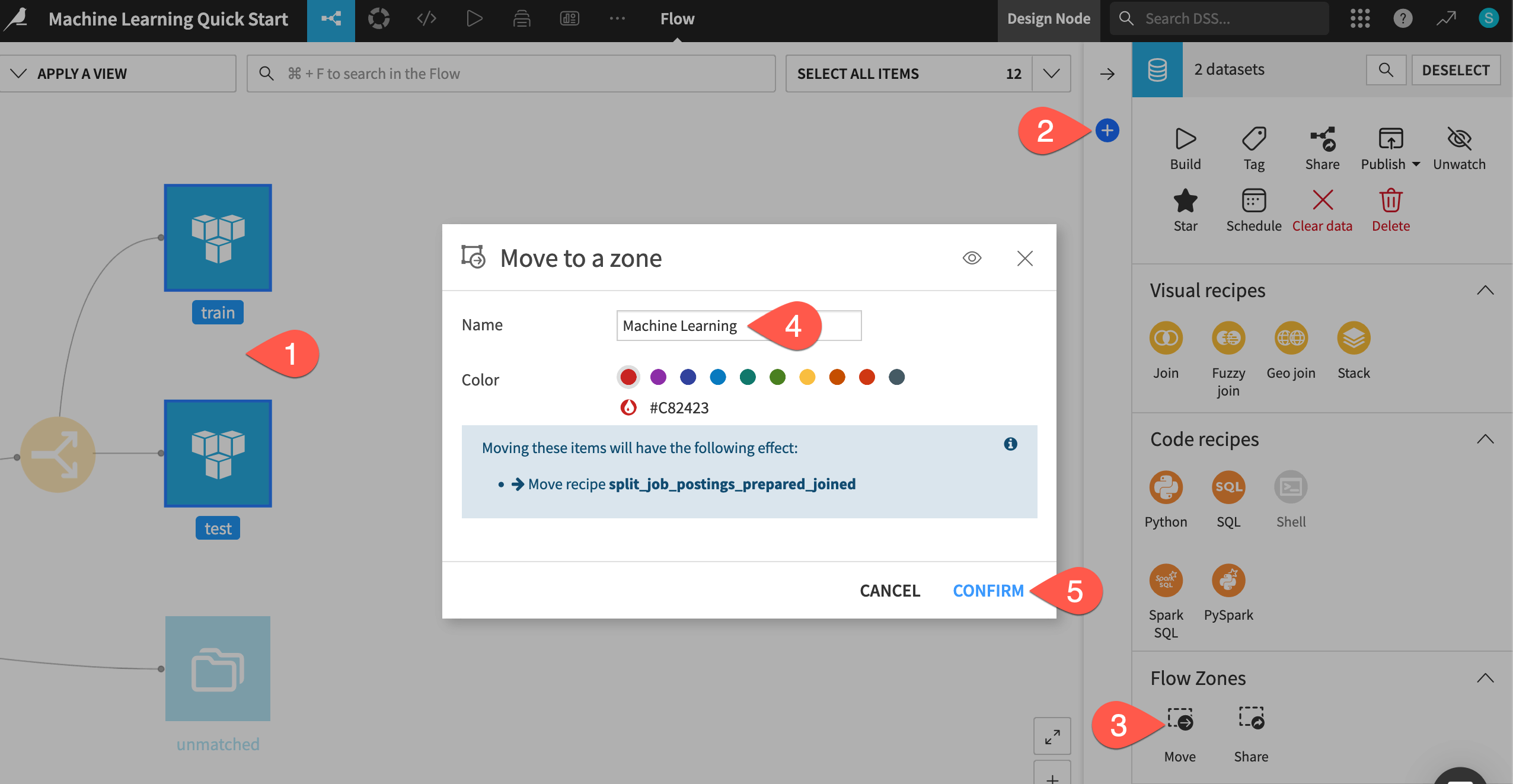
Create a separate Flow zone for the machine learning stage of this project.

Use the Cmd/Ctrl key and the cursor to select both the train and test datasets.
Open the Actions () tab of the right panel.
In the Flow Zones section, click Move.
Name the new zone Machine Learning.
Click Confirm.

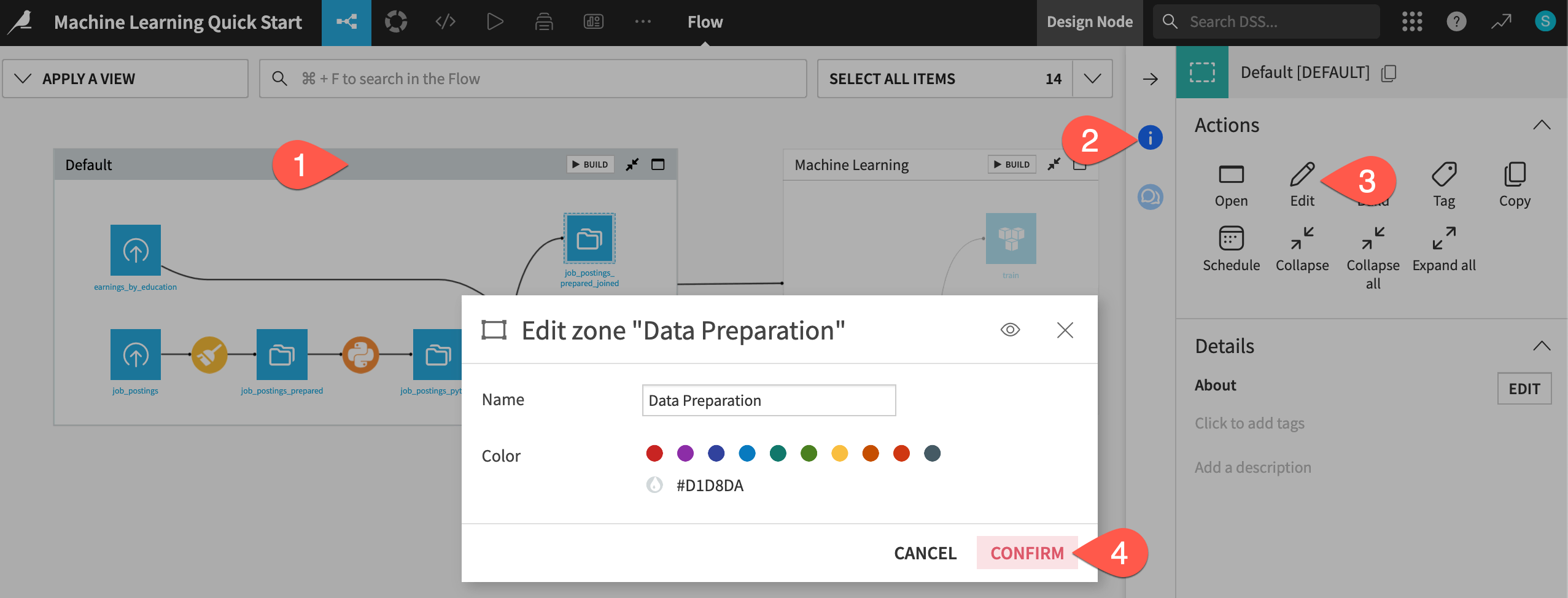
Now just rename the default zone, and you’ll have two clear spaces for these two stages of the project.

Click on the original Default zone.
Open the Actions () tab.
Select Edit.
Give the name Data Preparation.
Click Confirm.

Train machine learning models#

Now that the train and test data are in a separate Flow zone, let’s start creating models on the training data!

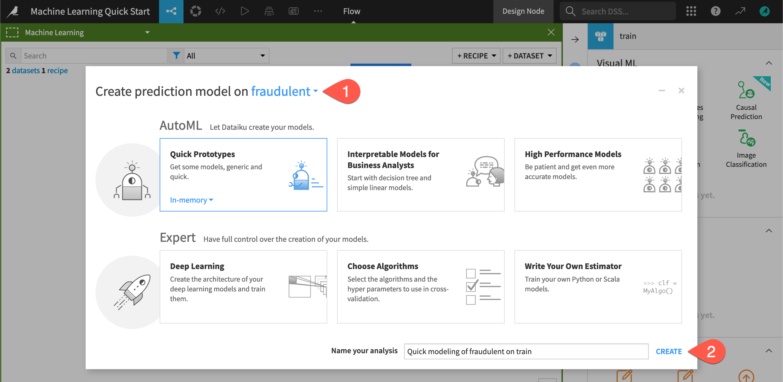
Create an AutoML prediction task#

The first step is to define the basic parameters of the machine learning task at hand.

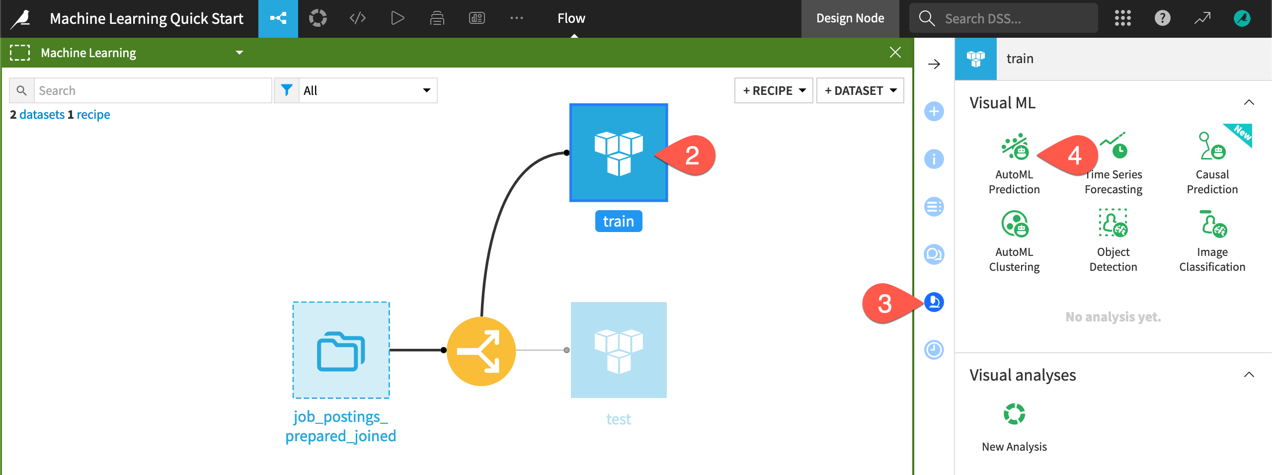
Click the top-right corner () of the Machine Learning Flow zone to open it.
Select the train dataset.
Navigate to the Lab () tab of the right side panel.
Among the menu of visual ML tasks, select AutoML Prediction.

Now you just need to choose the target variable and which kind of models you want to build.

Choose fraudulent as the target variable on which to create the prediction model.
Keeping the default setting of Quick Prototypes, click Create.

Important

In addition to AutoML Prediction shown here, you can build many other types of models in a similar manner. Among visual options, you could also build time series, clustering, image classification, object detection, or causal prediction models.

You can also mix code for custom preprocessing or custom algorithms into visual models. Alternatively, those wanting to go the full code route should explore the Developer Guide.

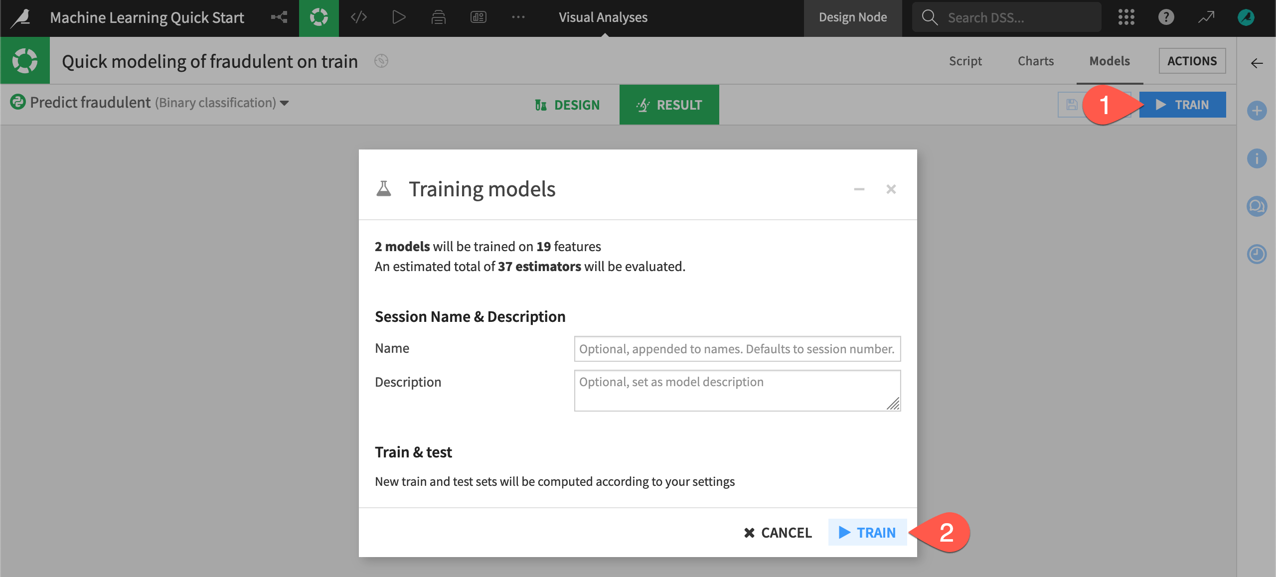
Train models with the default design#

Based on the characteristics of the input training data, Dataiku has automatically prepared the design of the model. But you haven’t trained any models yet!

Before adjusting the design, click Train to start a model training session.
Click Train again to confirm if necessary.

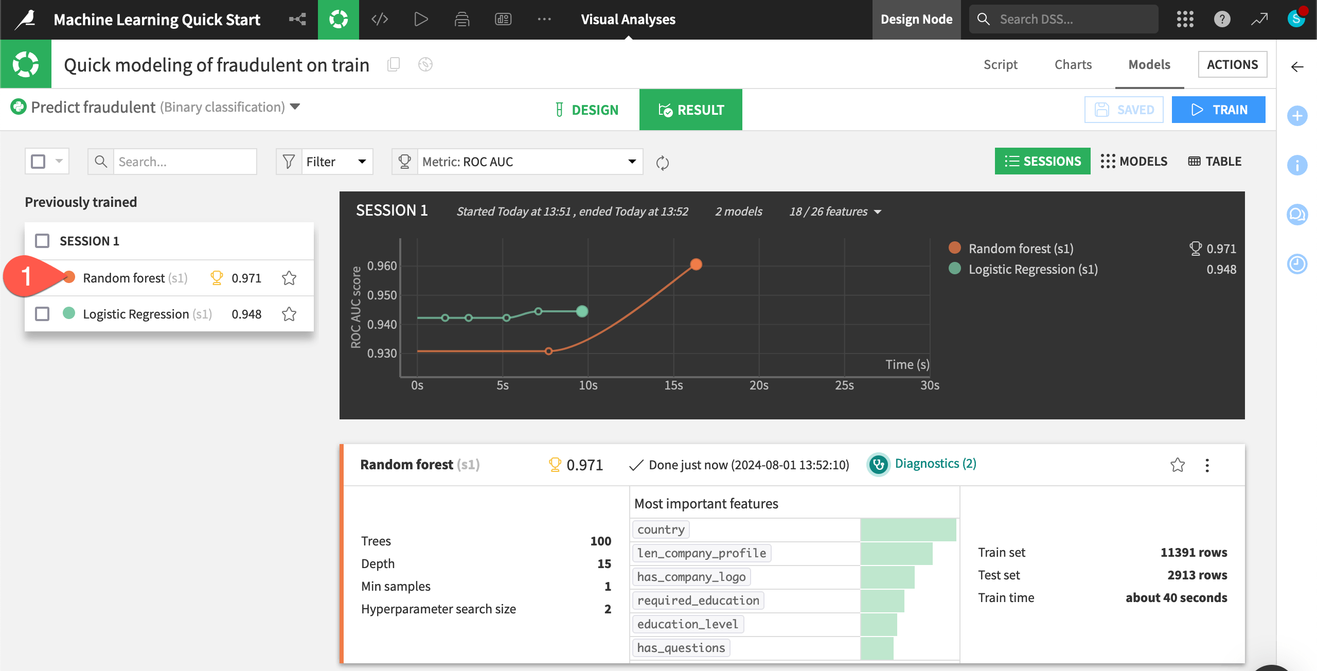
Inspect a model’s results#

Once your models have finished training, let’s see how Dataiku did.

While in the Result tab, click on the Random forest model in Session 1 on the left hand side of the screen to open a detailed model report.

Check model explainability#

One important aspect of a model is the ability to understand its predictions. The Explainability section of the report includes many tools for doing so.

In the Explainability section, click Feature importance to see an estimate of the influence of a feature on the predictions.

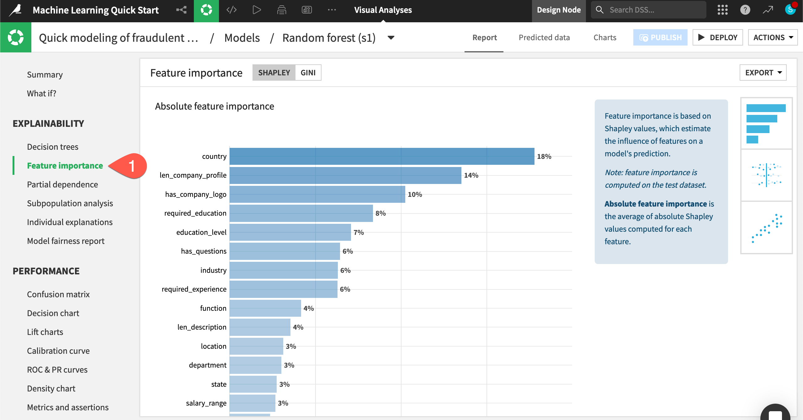
Note

Due to the somewhat random nature of algorithms like random forest, you might not have exactly the same results throughout this modeling exercise.

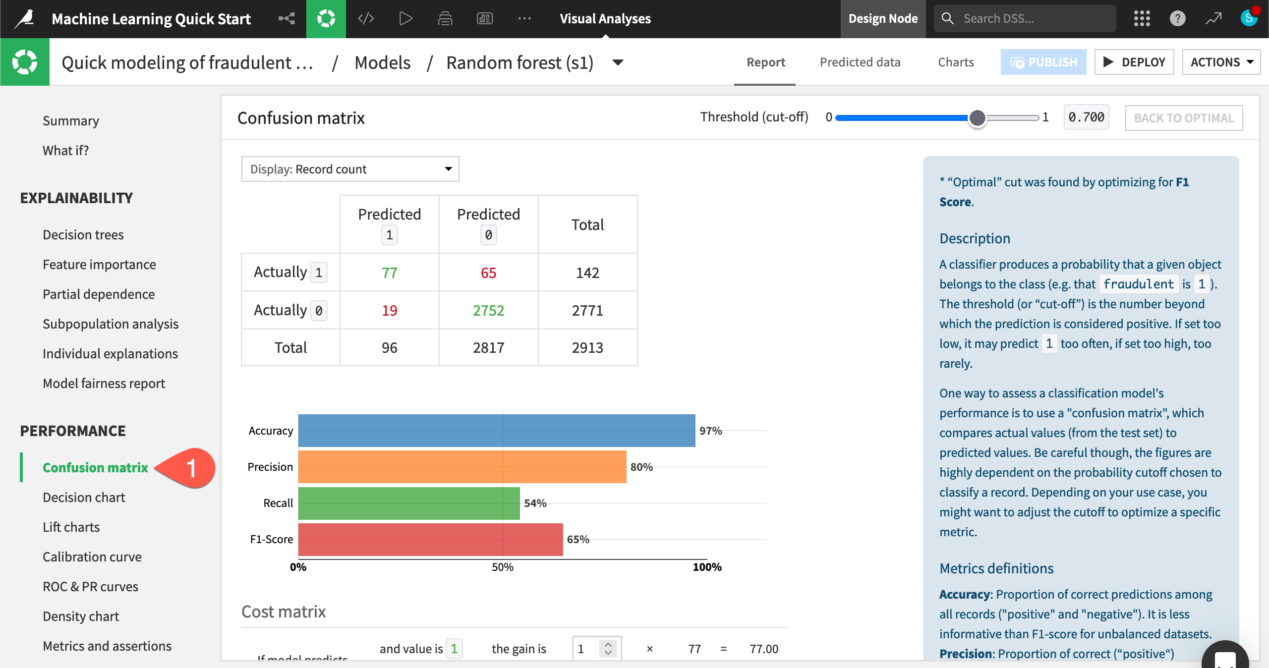
Check model performance#

You’ll also want to dive deeper into a model’s performance, starting with basic metrics for a classification problem like accuracy, precision, and recall.

In the Performance section, click Confusion matrix to check how well the model did at classifying real and fake job postings.

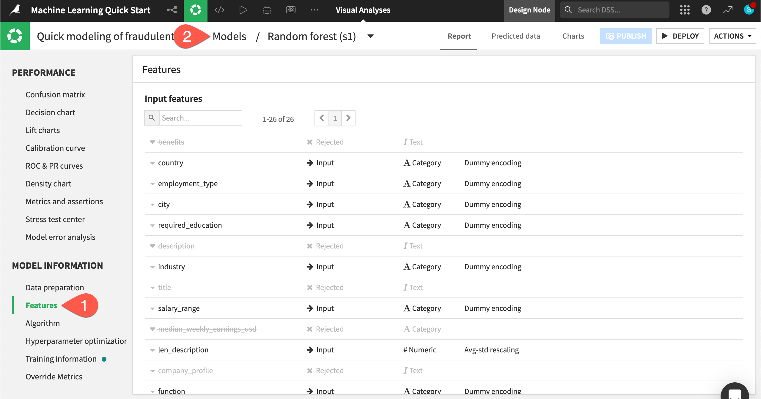
Check model information#

Alongside the results, you’ll also want to be sure how exactly the model was trained.

In the Model Information section, click Features to check which features were included in the model, which were rejected (such as the text features), and how they were handled.
When finished, click on Models to return to the Result home for the ML task.

Iterate on the design of a model training session#

Thus far, Dataiku has produced quick prototypes. From these baseline models, you can iteratively adjust the design, train new sessions of models, and then evaluate the results.

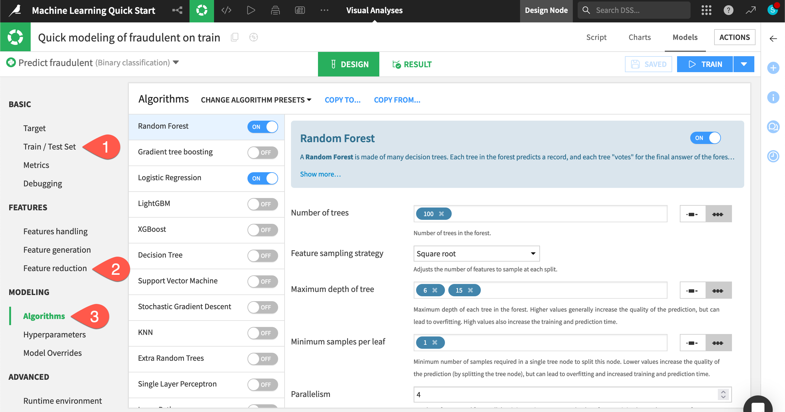
Switch to the Design tab.

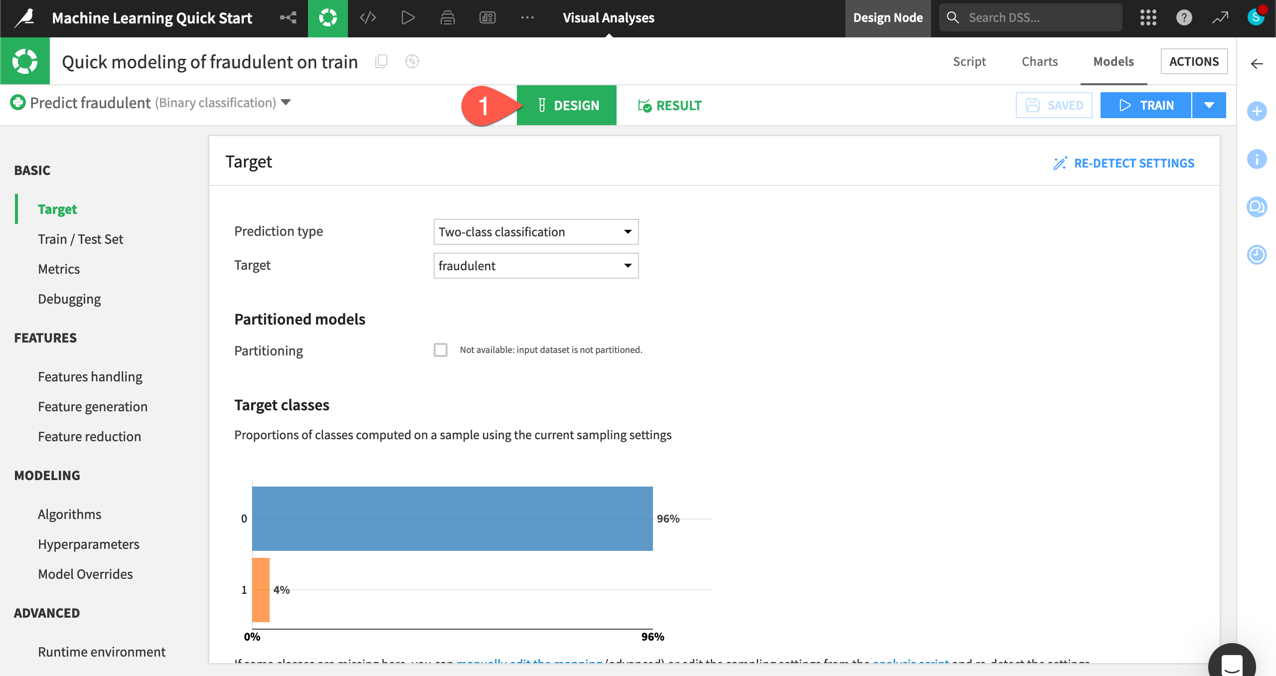
Tour the Design tab#

From the Design tab, you have full control over the design of a model training session. Take a quick tour of the available options. Some examples include:

In the Train / Test Set panel, you could apply a k-fold cross validation strategy.
In the Feature reduction panel, you could apply a reduction method like Principal Component Analysis.
In the Algorithms panel, you could select different machine learning algorithms or import custom Python models.

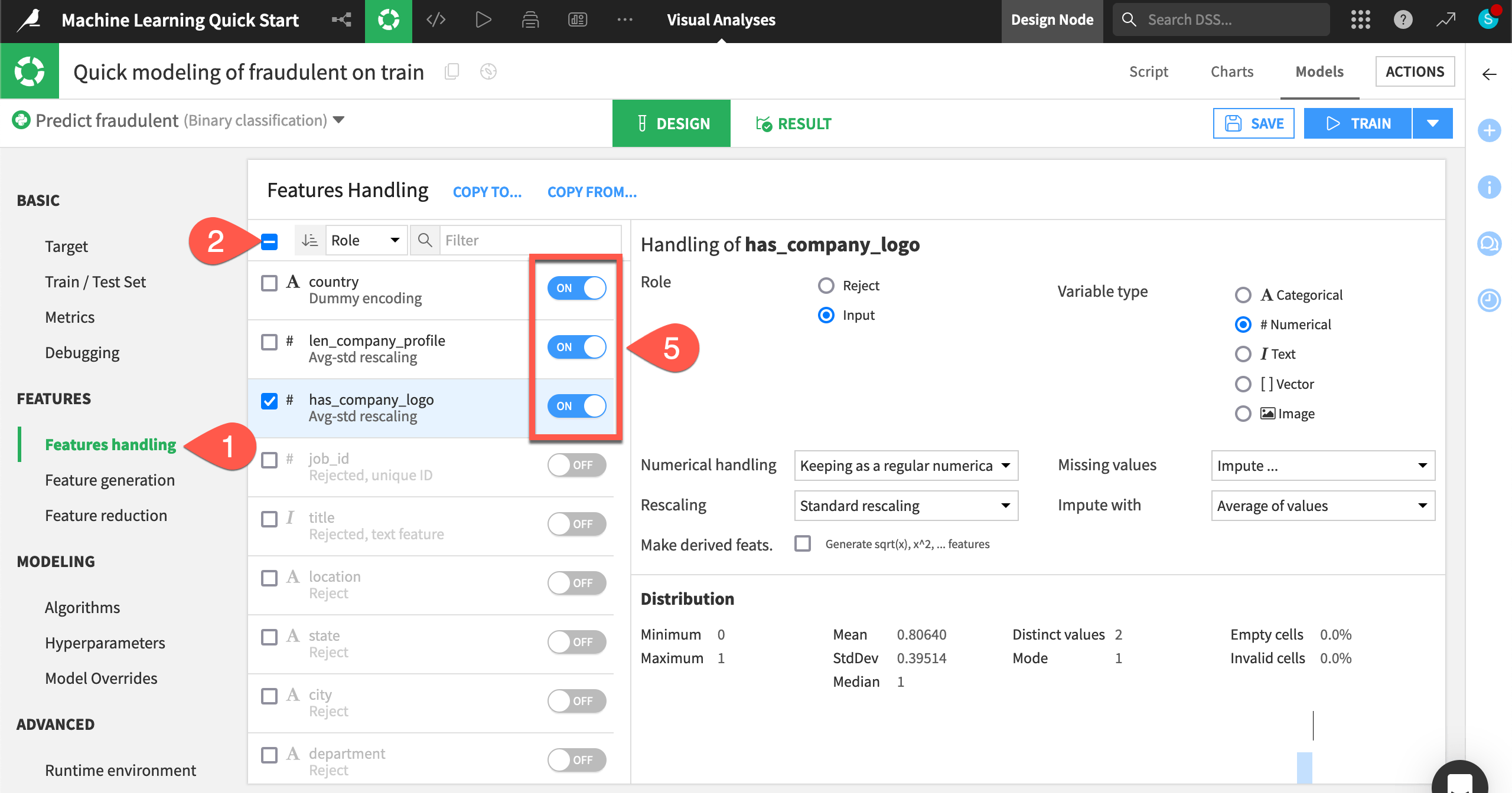
Reduce the number of features#

Instead of adding complexity, let’s simplify the model by including only the most important features. Having fewer features could hurt the model’s predictive performance, but it may bring other benefits, such as greater interpretability, faster training times, and reduced maintenance costs.

In the Design tab, navigate to the Features handling panel.
Click the box at the top left of the feature list to select all features.
For the role, click Reject to toggle off all features.
Click the box at the top left of the feature list to de-select all features.
Turn On the three most influential features according to the Feature importance chart seen earlier: country, len_company_profile, and has_company_logo.

Tip

Your top three features may be slightly different. Feel free to choose these three or the three most important from your own results.

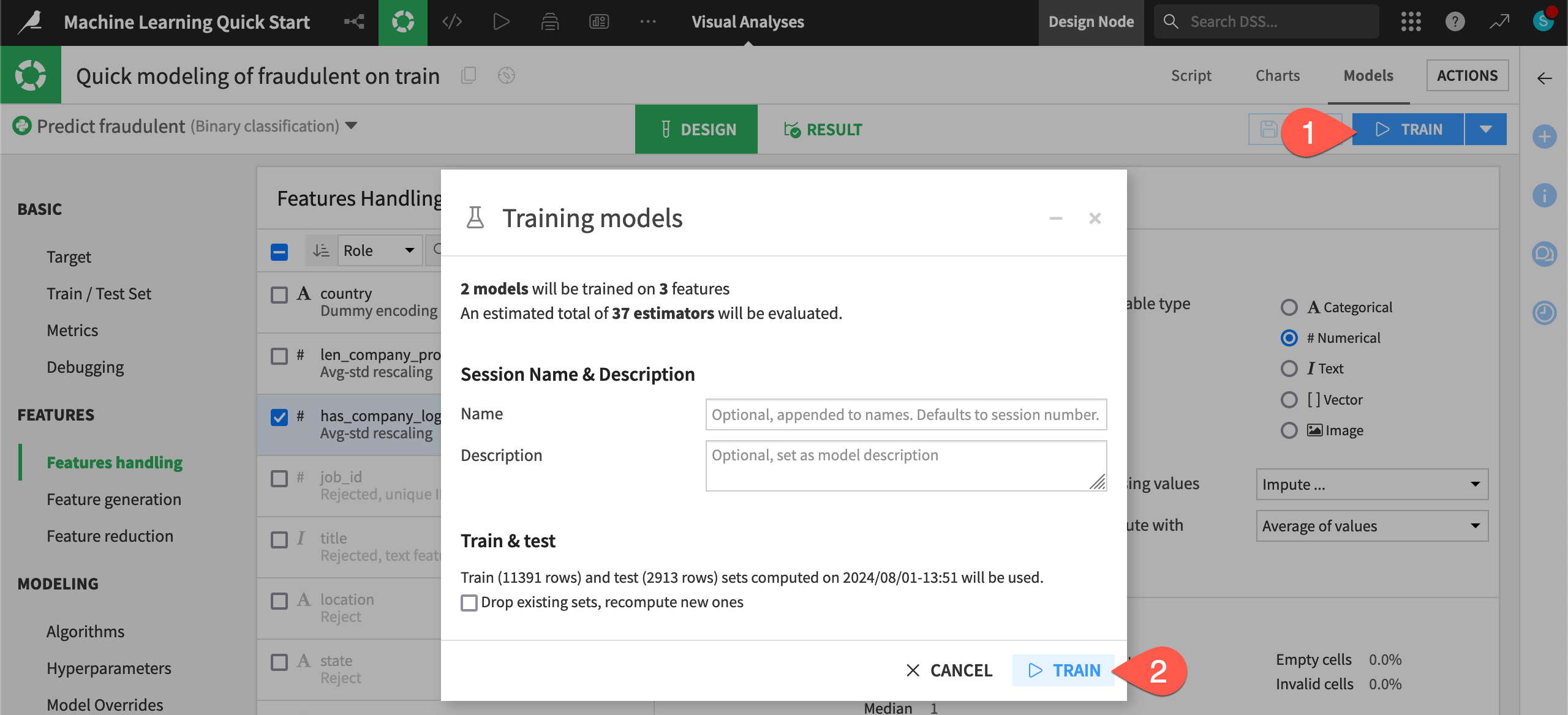
Train a second session#

Once you have just the top three features in the model design, you can kick off another training session.

Click Train.
Click Train once more to confirm.

Apply a model to generate predictions on new data#

Up until now, the models you’ve trained are present only in the Lab, a space for experimental prototyping and analysis. You can’t actually use any of these models until you have added them to the Flow. The Flow is where your actual project pipeline of datasets and recipes lives. Let’s do that now!

Choose a model to deploy#

Many factors could impact the choice of which model to deploy. For many use cases, the model’s performance isn’t the only deciding factor.

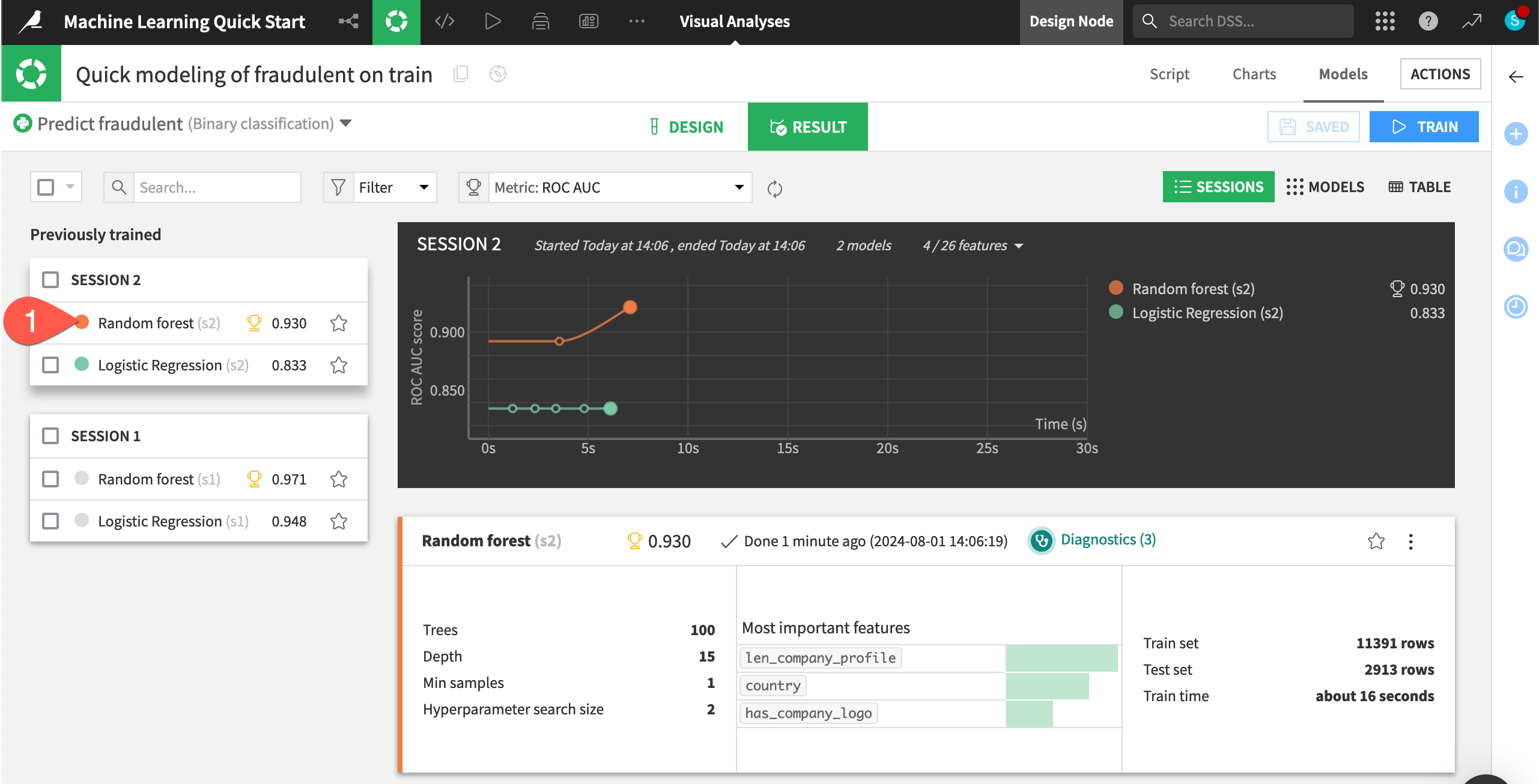
Compared to the larger model, the model with three features cost about 4 hundredths of a point in performance. For some use cases, this may be a significant difference. For others, it may be a bargain for a model that’s more interpretable, cheaper to train, and easier to maintain.

Since performance isn’t too important in this tutorial, choose the simpler option.

From the Result tab, click Random forest (s2) to open the model report of the simpler random forest model from Session 2.

Now you just need to deploy this model from the Lab to the Flow.

Click Deploy.
Click Create to confirm.

Explore a saved model object#

You now have two green objects in the Flow that you can use to generate predictions on new data: a training recipe and a saved model object.

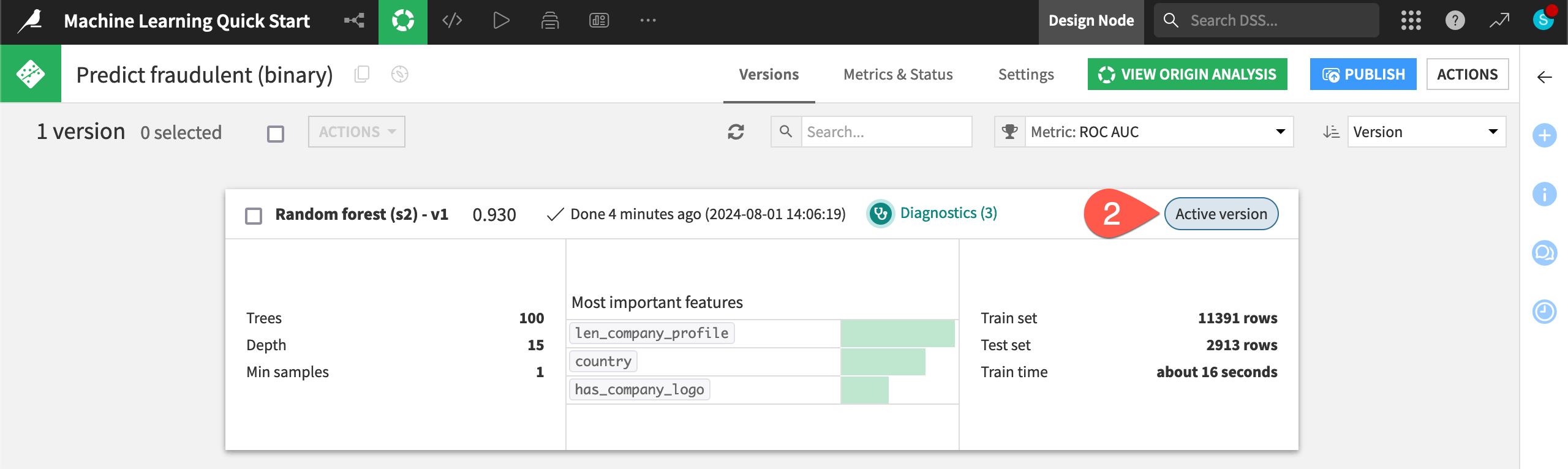
In the Machine Learning Flow zone, double click on the diamond-shaped saved model to open it.
Note the Active version label on the tile for the only version of this saved model.

Note

As you retrain the model, perhaps due to new data or additional feature engineering, you’ll deploy new active versions of the model to the Flow. However, you’ll still have the ability to revert to previous model versions at any time.

Score data#

Now let’s use the model in the Flow to generate predictions on a new dataset of job postings that the model hasn’t seen before.

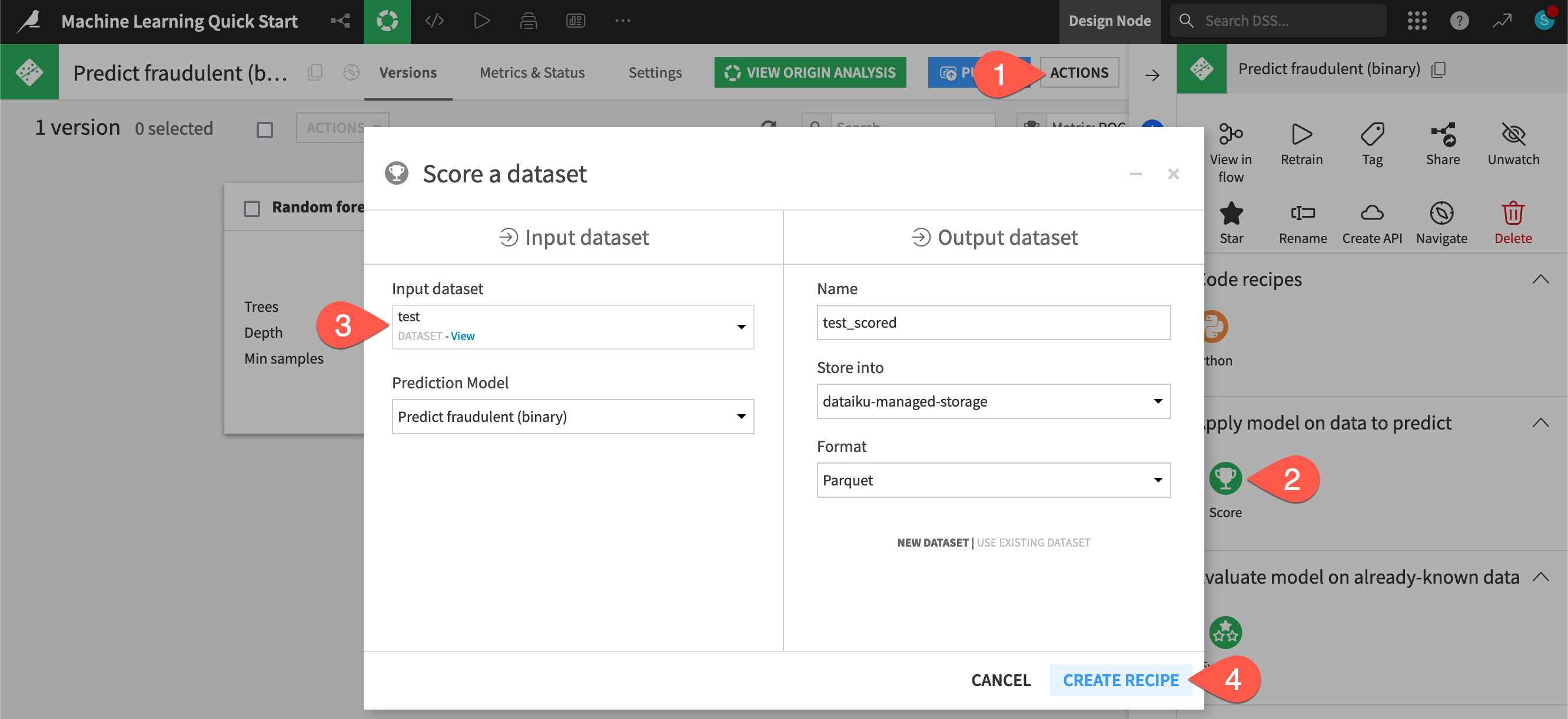
From the saved model screen, click to open the Actions () tab.
Select the Score recipe.
For the input dataset, select test.
Click Create Recipe, accepting the default output name.
Once on the Settings tab of the Score recipe, click Run (or type @ + r + u + n) to execute the recipe with the default settings.

Tip

Here you applied the Score recipe to a model trained with Dataiku’s visual AutoML. However, you also have the option to surface models deployed on external cloud ML platforms within Dataiku. Once surfaced, you can use them for scoring, monitoring, and more.

Inspect the scored data#

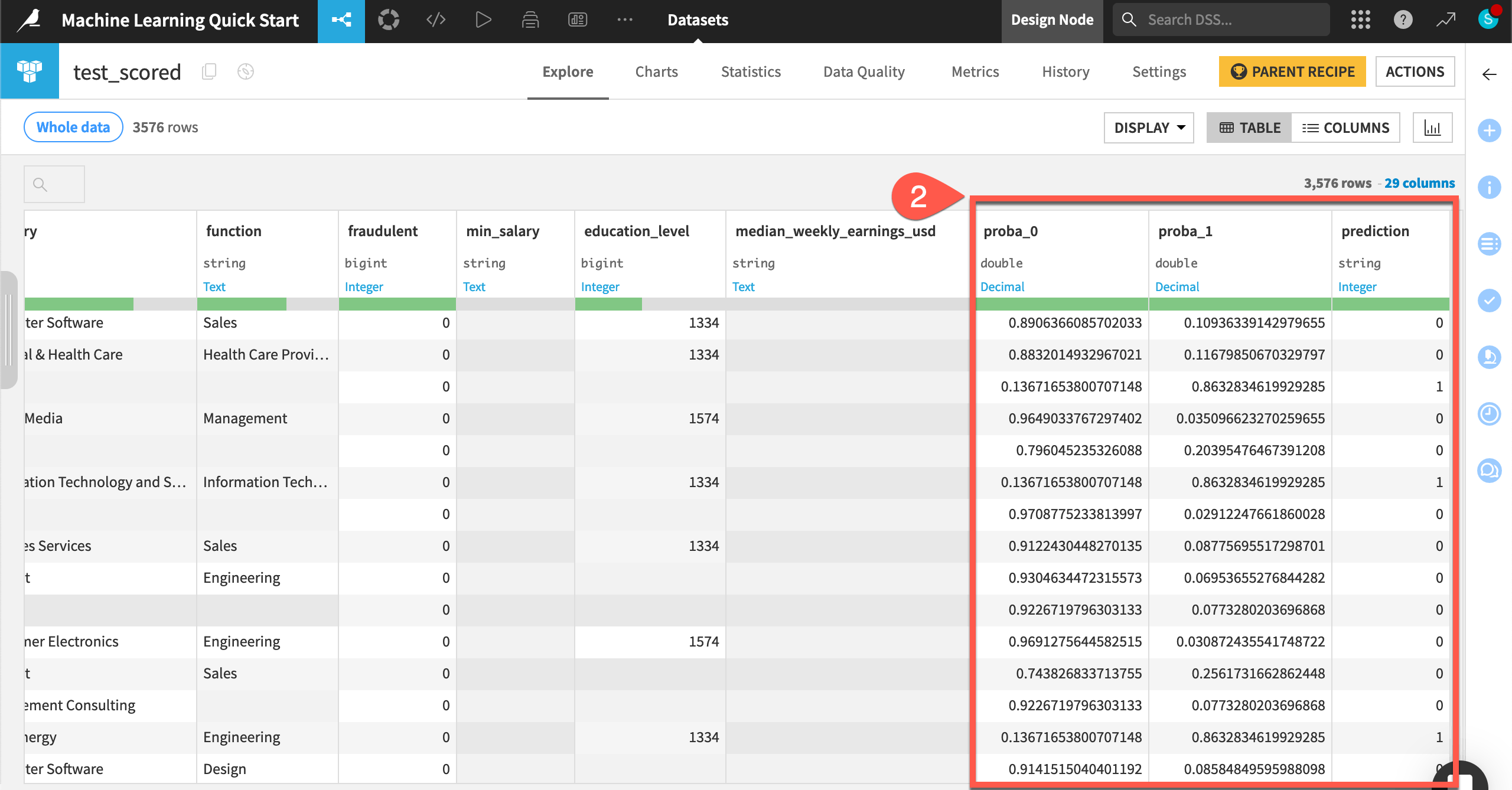
Compare the schemas of the test and test_scored datasets.

When the job finishes, click Explore dataset test_scored.
Note the addition of three new columns: proba_0, proba_1, and prediction.
Navigate back to the Flow (g + f) to see the scored dataset in the pipeline.

Tip

How well was the model able to identify the fake job postings in the test dataset? That’s a task for the Evaluate recipe, which you will encounter in other learning resources, such as the MLOps Practitioner learning path.

Next steps#

Congratulations! You’ve taken your first steps toward training machine learning models with Dataiku and using them to score data.

If you’ve already explored the Core Designer learning path, you’ll want to begin the ML Practitioner learning path and challenge yourself to earn the ML Practitioner certification.

Another option is to dive into the world of MLOps. In the Quick Start | Dataiku for MLOps, you can deploy an API endpoint from the model you’ve just created, and use it to answer real-time queries.