
Model metrics and explainability#
In the previous Introduction lesson, we created and trained a model to detect microcontrollers in images. In this lesson, we’ll view metrics to understand the model and its performance.
Model summary#
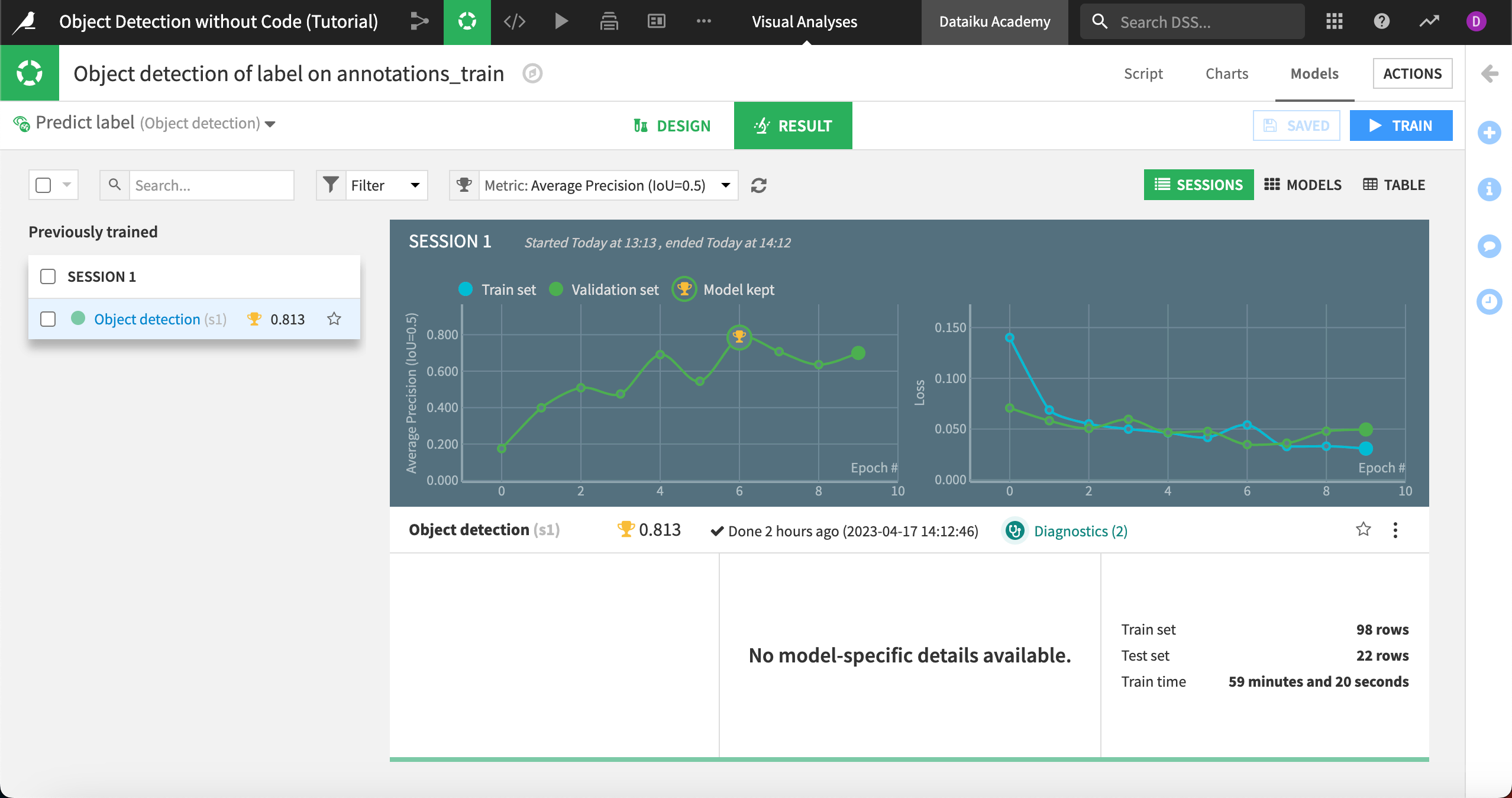
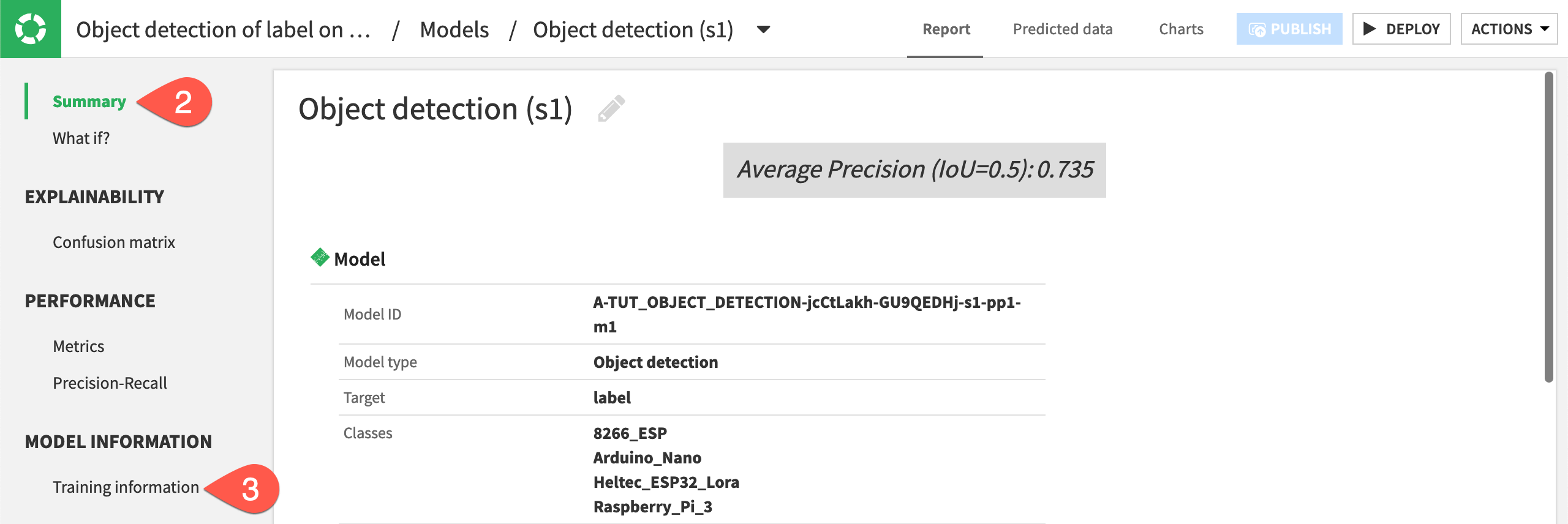
From the Result tab, click on the model name to navigate to the model report.
The Summary shows a report of the model’s training information, including the classes, epochs trained, and other parameters. Our model had an average precision of .813 (your results will vary). As we’ll see, the closer to 1 this number is, the stronger the model.
We can also view a number of other metrics.
What if#
You can upload new images directly into the model to find objects, classify them, and view the probabilities of each class. This information can give you insight into how the algorithm works and potential ways to improve it.
To see how this works, we’ll input a new image our model has not seen before.
Download the file
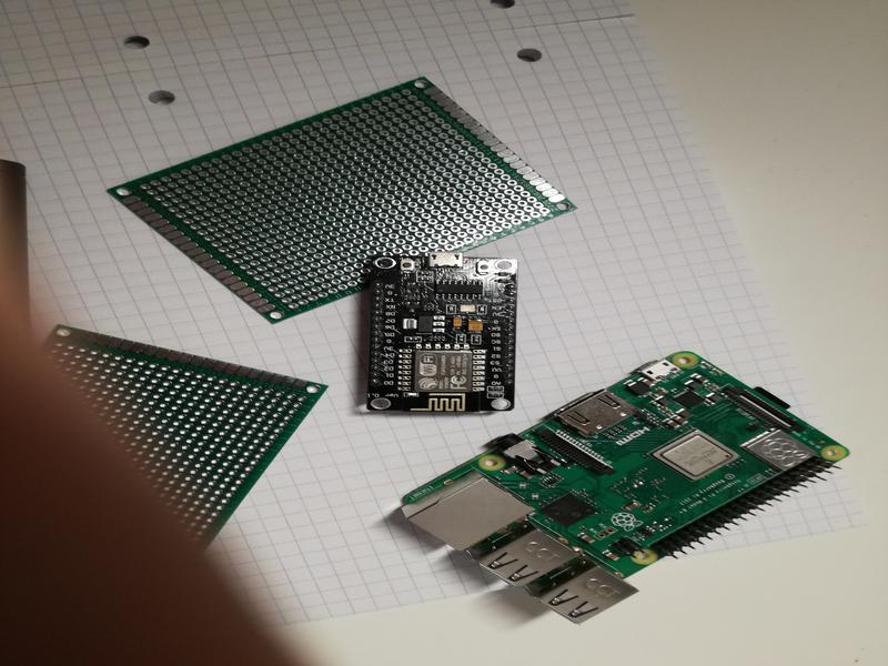
microcontroller_what-if, which is an image that contains two controllers — a Raspberry Pi and a ESP8266.Navigate to What if? on the left panel.
Either drag and drop the new image onto the screen or click Browse for images and find the image to upload.
The model correctly identifies both controllers in the image, with a relatively high confidence for the Raspberry Pi but lower confidence of about 66% for the ESP. We also do not see any false positive detections on other objects in the image.
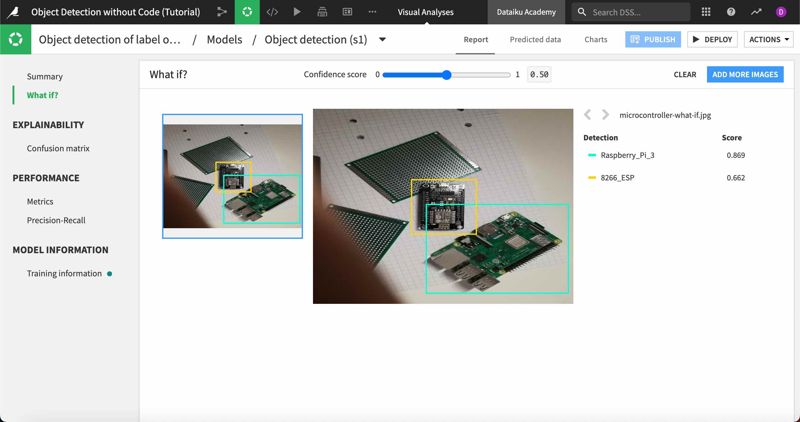
You can hover over the class names on the right to highlight the detected objects in the image. You also may upload more images to the What if? panel.
Explainability#
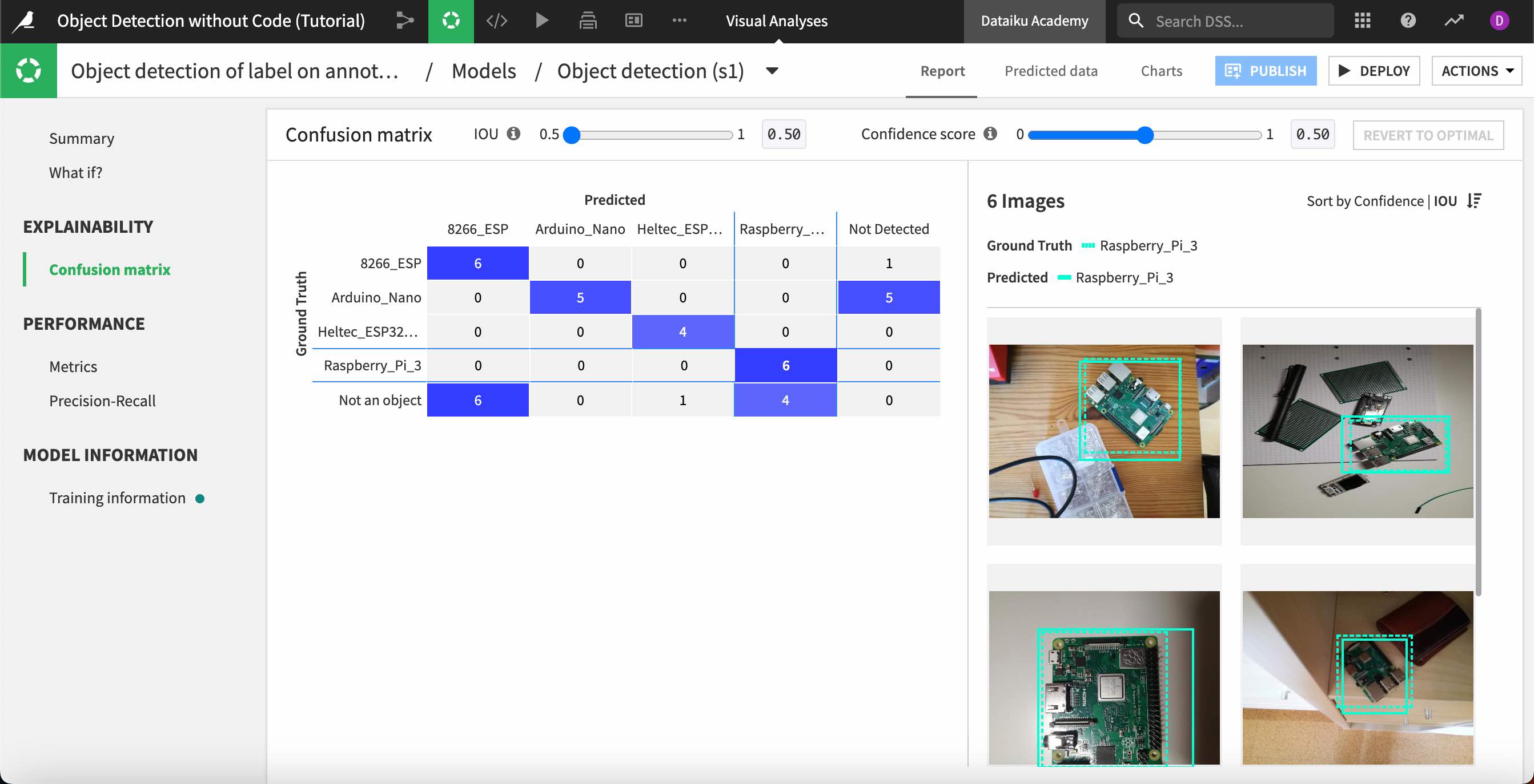
Dataiku calculates the number of true positive and false positive detections in the testing set of images, then inputs those values into a confusion matrix.
Navigate to the Confusion matrix panel under Explainability.
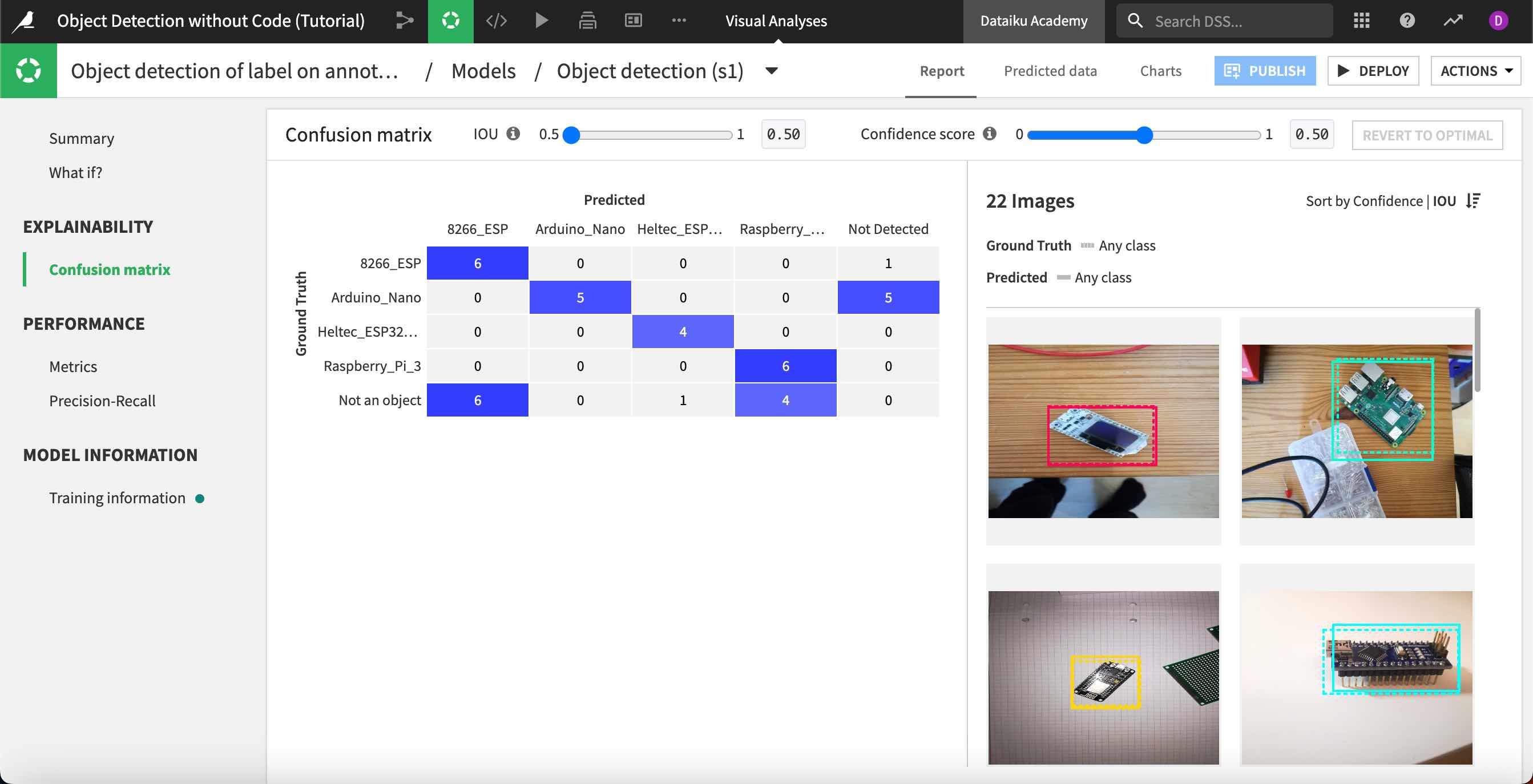
Though your results will vary, we can see in this example that the model correctly predicted six of the ESP8266 chips, but did not detect one of them. It also detected six objects that were not the microchips (in the “Not an object” row) and classified them as an ESP8266.
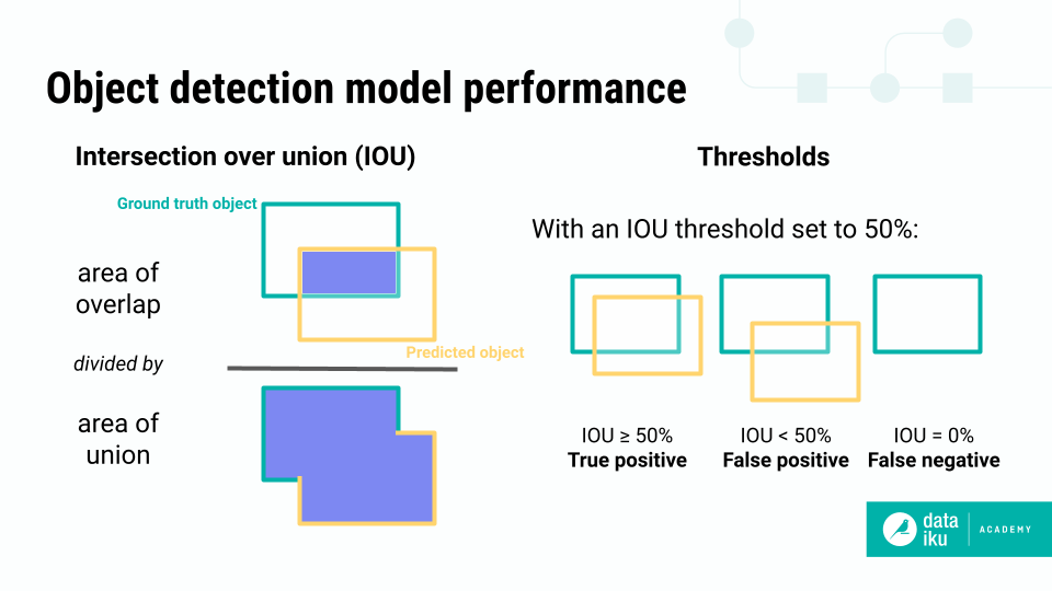
The true and false positive calculations in the confusion matrix are based on two measures: the Intersection over union, or IOU, and the Confidence score.
The Confidence score is the probability that a predicted box contains the predicted object.
IOU is a measure of the overlap between the model’s predicted bounding box and the ground truth bounding box provided in the training images. By comparing the IoU to an overlap threshold that you set, Dataiku can tell if a detection is correct (a true positive), incorrect (a false positive), or completely missed (a false negative).
The IOU threshold is the lowest acceptable overlap for a detection to be considered a true positive. For example, with a threshold of 50%, the model’s detected object must overlap the true object by 50% or more to be considered a true detection. If a detection overlaps by only 40%, it would be considered a false positive.
You can change the IOU and confidence score at the top of the confusion matrix. Experiment with different settings and note how the values in the matrix change.
We can see that moving the threshold and confidence score higher means the model misses many more predictions. In fact, in our example, it missed all of the Arduino objects and nearly all of the others.
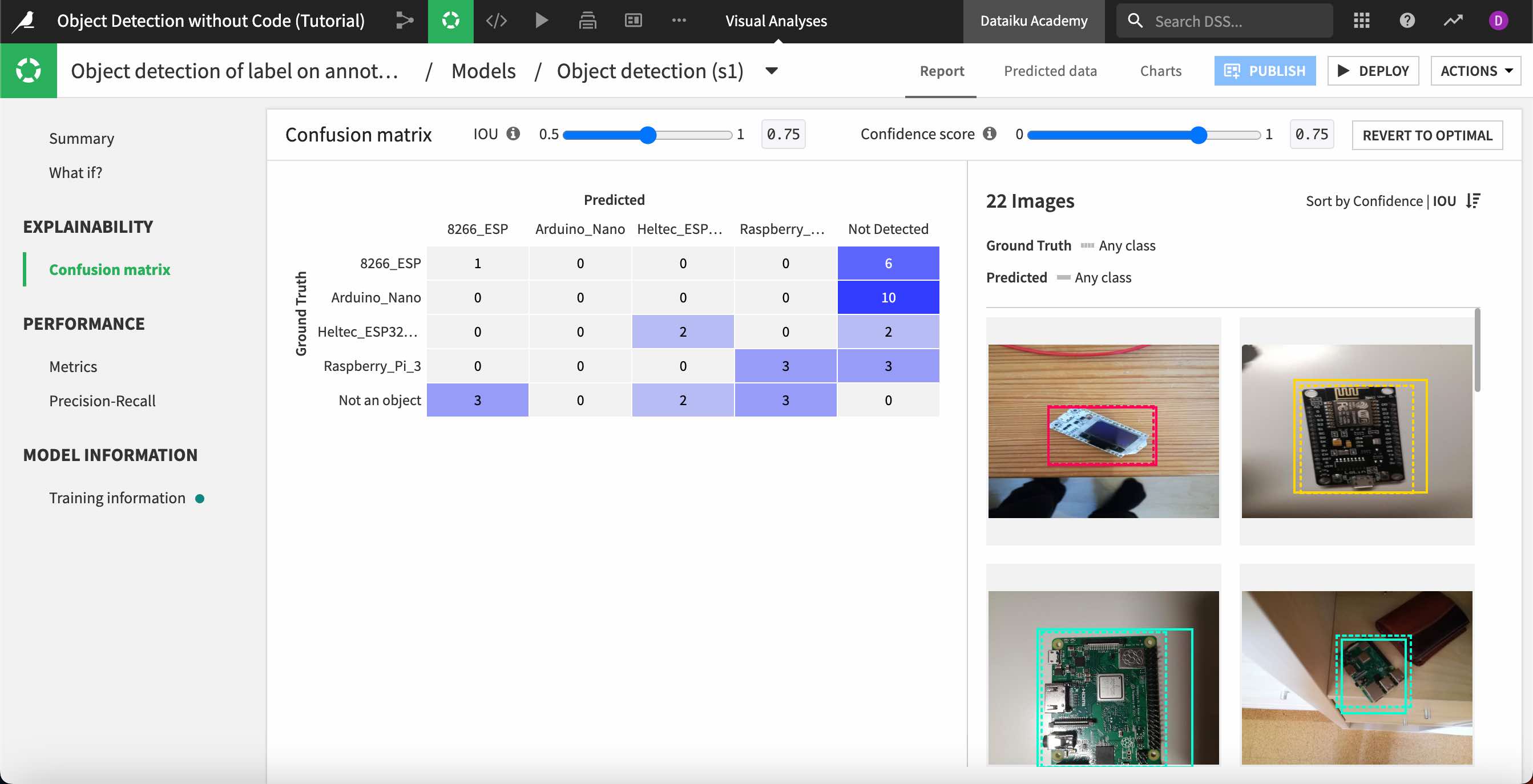
You can return to the optimal settings with the button at the top right.
Double click on any image on the right to view the ground truth and predicted object bounding boxes, the object class, and confidence level. You can filter the images displayed by clicking on any value in the confusion matrix. For example, click on the cell representing the Raspberry Pi true positive detections.
Performance#
Navigate to the Metrics panel under Performance, where we can view detailed information about the model’s performance for each type of object.
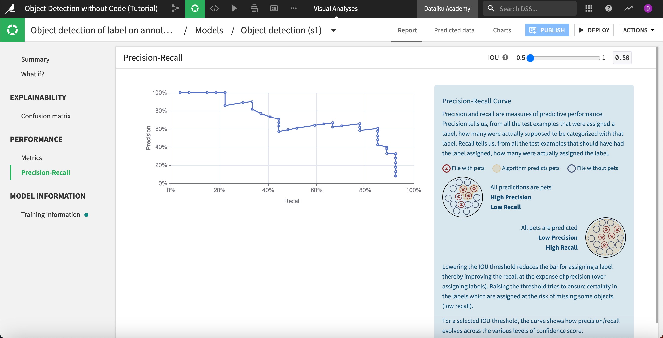
The evaluation metric is Average precision, which measures how well your model performs. The closer to 1 this score is, the better your model is performing on the test set. The average precision measures the area under the precision-recall curve, which you can view under Precision-Recall.
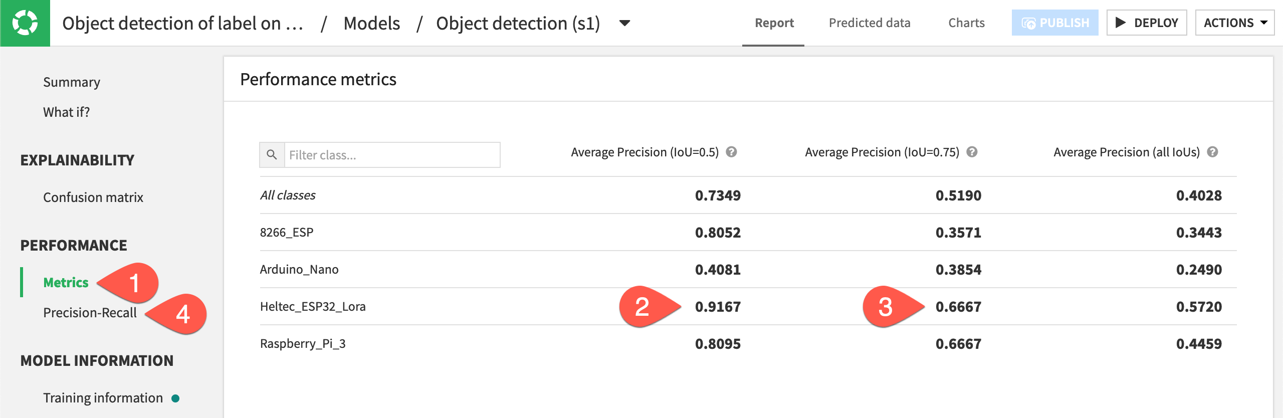
In this case, we can see that the model performed best when detecting Heltec ESP32 Lora controllers with an IOU of 50%. It makes sense that the model’s performance declines as the IOU increases, because the overlap threshold for counting a true positive detection is higher.