Tutorial | Predictive maintenance in the manufacturing industry#

Note

This content was last updated using Dataiku 11.

Overview#

Important

Please note that this tutorial is for learning purposes only. See Solution | Maintenance Performance and Planning for a pre-built project capability of solving problems in this industry.

Business case#

We are part of the data team of an important OEM company working on a predictive maintenance use case. Our goal is to create a system that, based on the vehicle’s sensor data, will trigger some preventive maintenance actions.

Unexpected problems on the road are very inconvenient to customers. With this in mind, the company wants to send a message to those cars that are more likely to break down before a problem occurs, thereby minimizing the chance of a car breaking down on a customer. At the same time, requesting otherwise healthy vehicles too often would not be cost-effective either.

The company has some information on past failures, as well as on car usage and maintenance. As the data team, we are here to offer a data-driven approach. More specifically, we want to use the information we have to answer the following questions:

What are the most common factors behind these failures?
Which cars are most likely to fail?

These questions are interrelated. As a data team, we are looking to isolate and understand which factors can help predict a higher probability of vehicle failure. To do so, we’ll build end-to-end predictive models in Dataiku. We’ll see an entire advanced analytics workflow from start to finish. Hopefully, its results will end up as a data product that promotes customer safety and has a direct impact on the company’s bottom line!

Supporting data#

We’ll need three datasets in this tutorial. Find their descriptions and links to download below:

usage: number of miles the cars have been driven, collected at various points;
maintenance: records of when cars were serviced, which parts were serviced, the reason for service, and the quantity of parts replaced during maintenance;
failure: whether a vehicle had a recorded failure (not all cases are labelled).

An Asset ID, available in each file, uniquely identifies each car. Some datasets are organized at the vehicle level; others are not. A bit of data detective work might be required!

Workflow overview#

By the end of this walkthrough, your workflow in Dataiku should mirror the one below.

In order to achieve this workflow, we will complete the following high-level steps:

Import the data.
Clean, restructure and merge the input datasets together.
Generate features.
Split the data by whether outcomes are known and unknown, i.e., labelled and unlabelled.
Train and analyze a predictive model on the known cases.
Score the unlabelled cases using the predictive model.
Batch deploy the project to a production environment (optional).

Prerequisites#

You should be familiar with:

Dataiku basics (Core Designer or equivalent)
Visual machine learning in Dataiku, such as in ML Basics

Technical requirements#

To complete this walkthrough, the following requirements need to be met:

Have access to a Dataiku instance–that’s it!
If you plan to also batch deploy the project (the final step in our end-to-end pipeline), you’ll also need an Automation node connected to your Design node.

Create the project and import datasets#

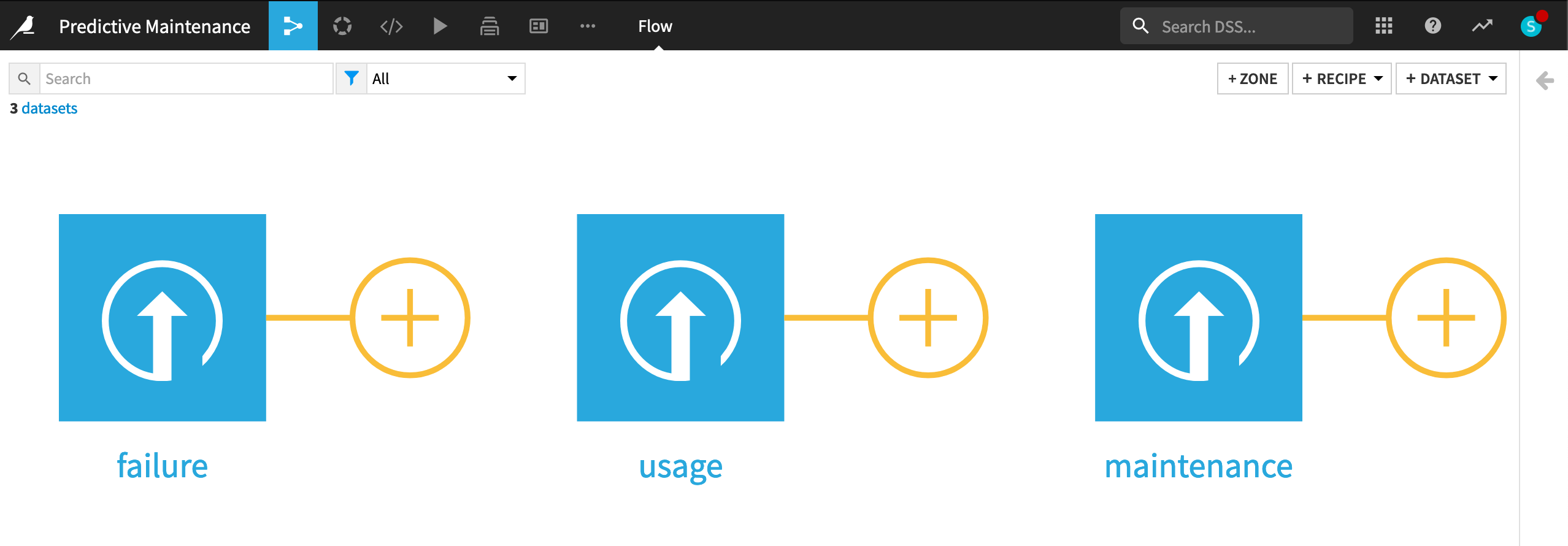
First, we will import three input files into Dataiku.

From the Dataiku homepage, click + New Project > Blank project.
Name it Predictive Maintenance.
Import the usage, maintenance, and failure datasets found in the “Supporting Data” section.

Note

To review how to import flat files, return to the Tutorial | Getting started with datasets.

Prepare the usage dataset#

The usage dataset tracks the mileage for cars, identified by their Asset ID, at a given point in Time.

The Use variable records the total number of miles a car has driven at the specified Time.
The units of the Time variable are not clear. Perhaps days from a particular date? You could start a discussion with the data’s owner to find out.
Here Asset ID is not unique, i.e., the same car might have more than a single row of data.

After importing the CSV file, from the Explore tab, we can see that the columns are stored as “string” type (the gray text beneath the column header), even though Dataiku can infer from the sample the meanings to be “Text”, “Integer”, and “Decimal” (the blue text beneath the storage type).

Note

For more on the distinction between storage types and meanings, please see the reference documentation or the concept lessons on schema, storage type and meanings.

Accordingly, with data stored as strings, we won’t be able to perform any mathematical operations on seemingly-numeric columns, such as Use. Let’s fix this.

Navigate to the Settings > Schema tab, which shows the storage types and meanings for all columns.
Click Check Now to determine that the schema and data are consistent.
Then click Infer Types from Data to allow Dataiku to assign new storage types and high-level classifications.
Save the changes.

Returning to the Explore tab, note that although the meanings (written in blue) have not changed, the storage types in gray have updated to “string”, “bigint”, and “double”.

Note

As noted in the UI, this action only takes into account the current sample, and so should be used cautiously. There are a number of different ways to perform type inference in Dataiku, each with their own pros and cons, depending on your objectives. Initiating a Prepare recipe, for example, is another way to instruct Dataiku to perform type inference. For more information, see the reference documentation on creating schemas of datasets.

For most individual cars, we have many Use readings at many different times. However, we want the data to reflect the individual car so that we can model outcomes at the vehicle-level. Now with the correct storage types in place, we can process the dataset with a Group By recipe.

From the usage dataset, initiate a Group By recipe from the Actions menu.
Choose to Group By Asset in the dropdown menu.
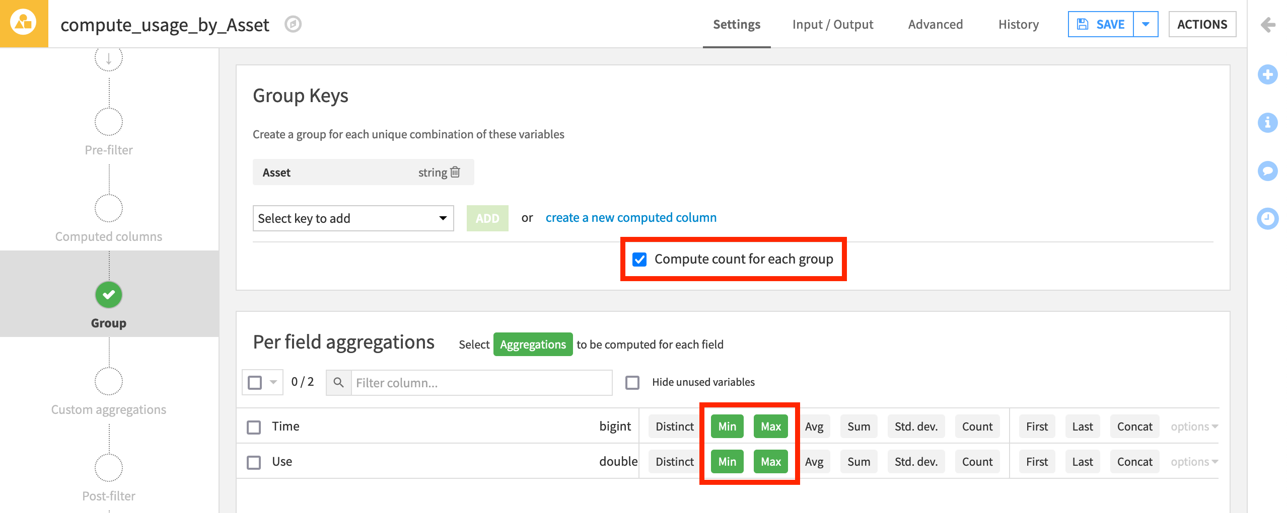
Keep the default output dataset name usage_by_Asset.
In the Group step, we want the count for each group (selected by default).
Add to this the Min and Max for both Time and Use.
Run the recipe.

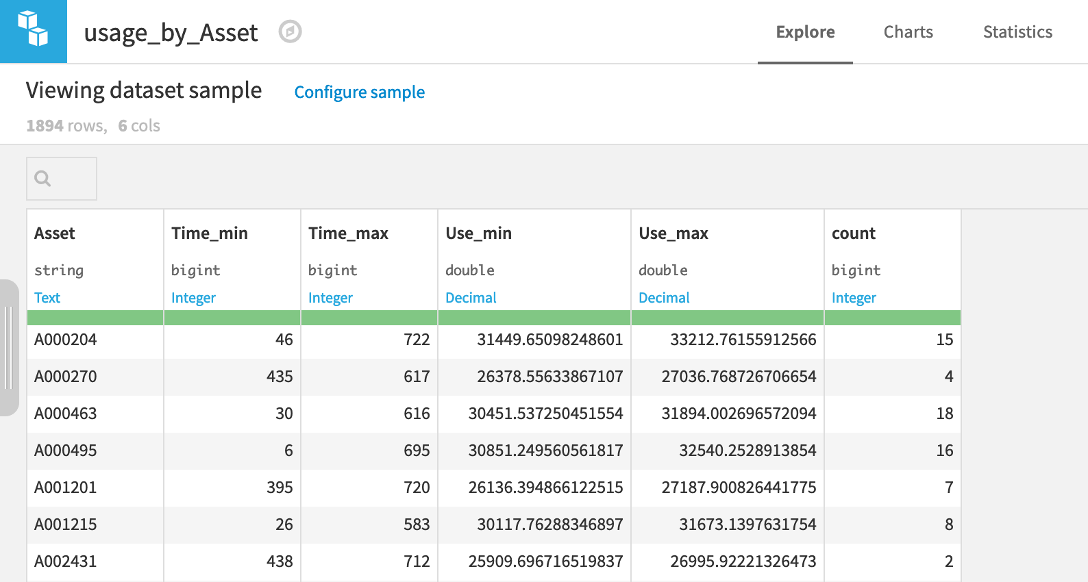
Now aggregated at the level of a unique car, the output dataset is fit for our purposes.

Let’s see if the maintenance dataset can be brought to the same level.

Prepare the maintenance dataset#

The maintenance dataset documents activity that has occurred with respect to a given Asset, organized by Part (what was repaired) and Time (when it was repaired). A Reason variable codifies the nature of the problem.

As we did for the usage dataset, we want to organize the maintenance dataset to the level of unique vehicles. For the usage dataset, we achieved this with the Group recipe. Here, we’ll use the Pivot recipe.

While the current dataset has many observations for each vehicle, we need the output dataset to be “pivoted” at the level of each vehicle; that is, transformed from narrow to wide.

As done for the usage dataset, infer storage types so that the variables Time and Quantity are no longer stored as strings.
Next, use the Pivot recipe to restructure the dataset at the level of each vehicle. In detail:
- With maintenance chosen as the input dataset, choose to Pivot By Reason.
- Keep the default output dataset name maintenance_by_Reason, and Create Recipe.
- At the Pivot step, select Asset as the “Row identifier”.
- Reason should already be selected under Create columns with. Although it should make no difference in this case, change Pivoted values to all so that all values of Reason are pivoted into columns.
- Populate content with the sum of Quantity.
- Deselect “Count of records”.
Run the recipe.

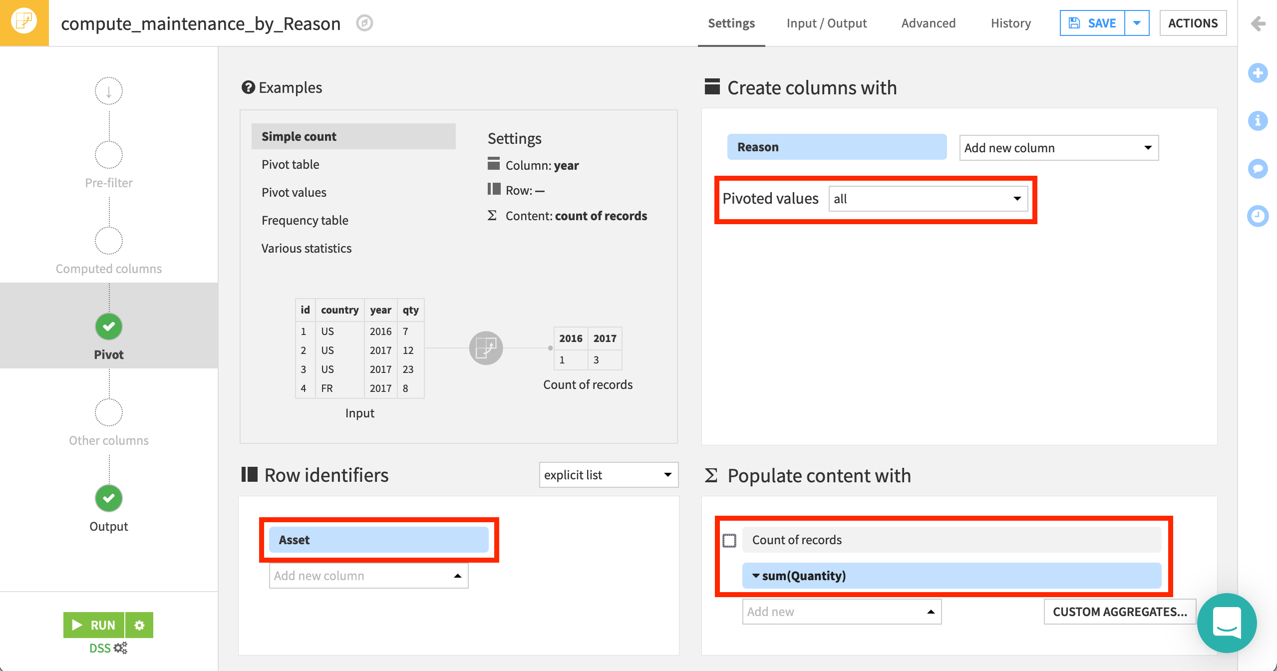
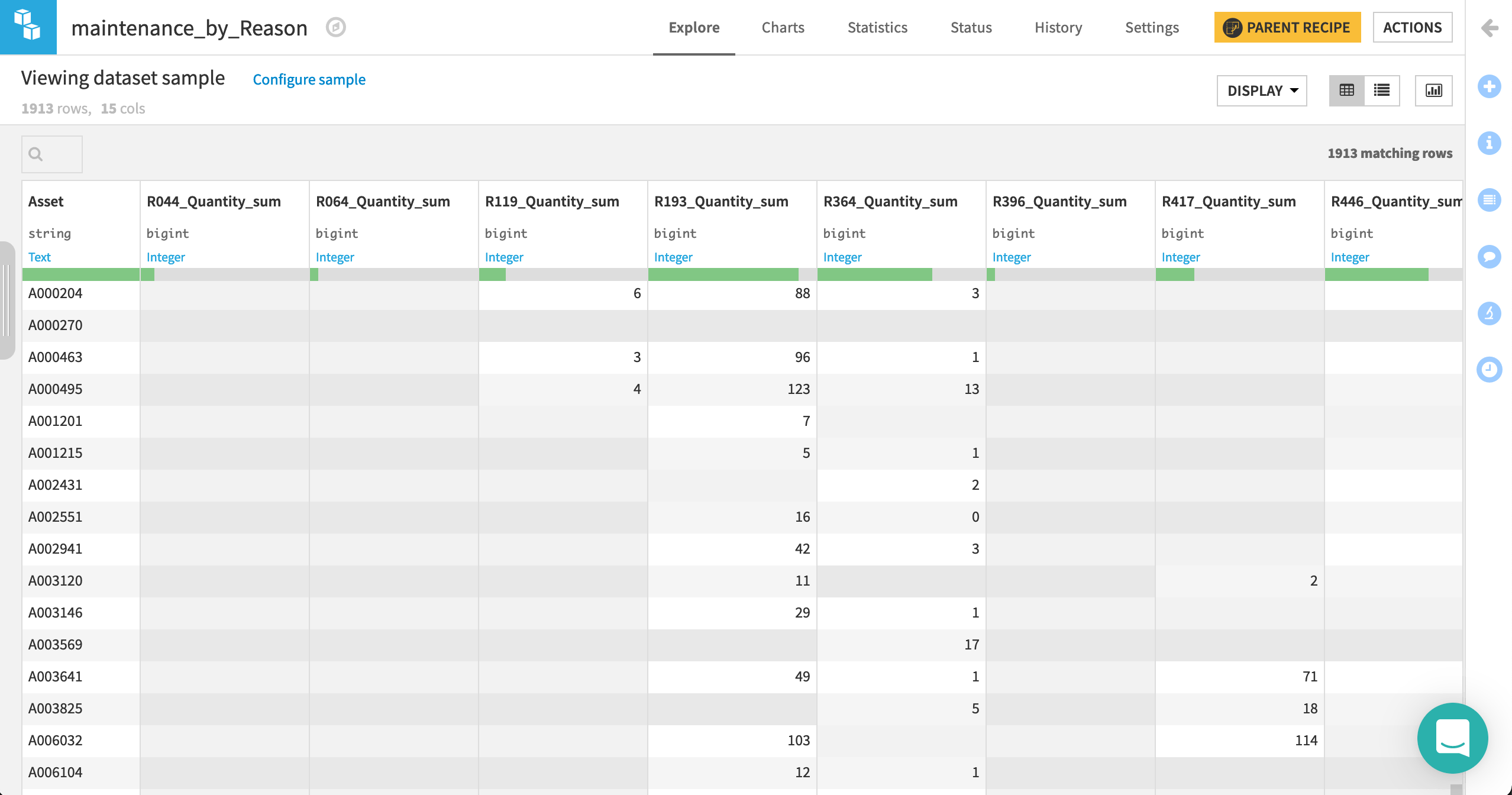
The 14 distinct reasons are now spread across their own columns, with one asset per row.

Note

More detailed information on the Pivot recipe, such as how it computes the output schema, can be found in Concept | Pivot recipe.

Prepare the failure dataset#

The failure dataset has only two columns: Asset and failure_bin.

Here Asset IDs are unique (i.e., one row for each ID), so we are already structured at the level of individual cars. The Analyze tool is one quick method to verify this property.
The failure_bin column is the target variable. A score of 1 represents the failure of the associated Asset. We can use this variable as a label to model predictions for failures among the fleet.

Only one preparation step is needed here.

As done with the previous two datasets, Infer Types from Data within the Settings > Schema tab so that failure_bin is stored as a bigint.

Next, we’ll join all of our datasets together!

Join the datasets#

We now have three datasets at the same level of granularity: the Asset, i.e., an individual car. Joining them together will give us the most possible information for a model. With the same Asset ID in each dataset, we can easily join the datasets with a visual recipe.

From the failure dataset, initiate a Join recipe.
Add usage_by_Asset as the second input dataset.
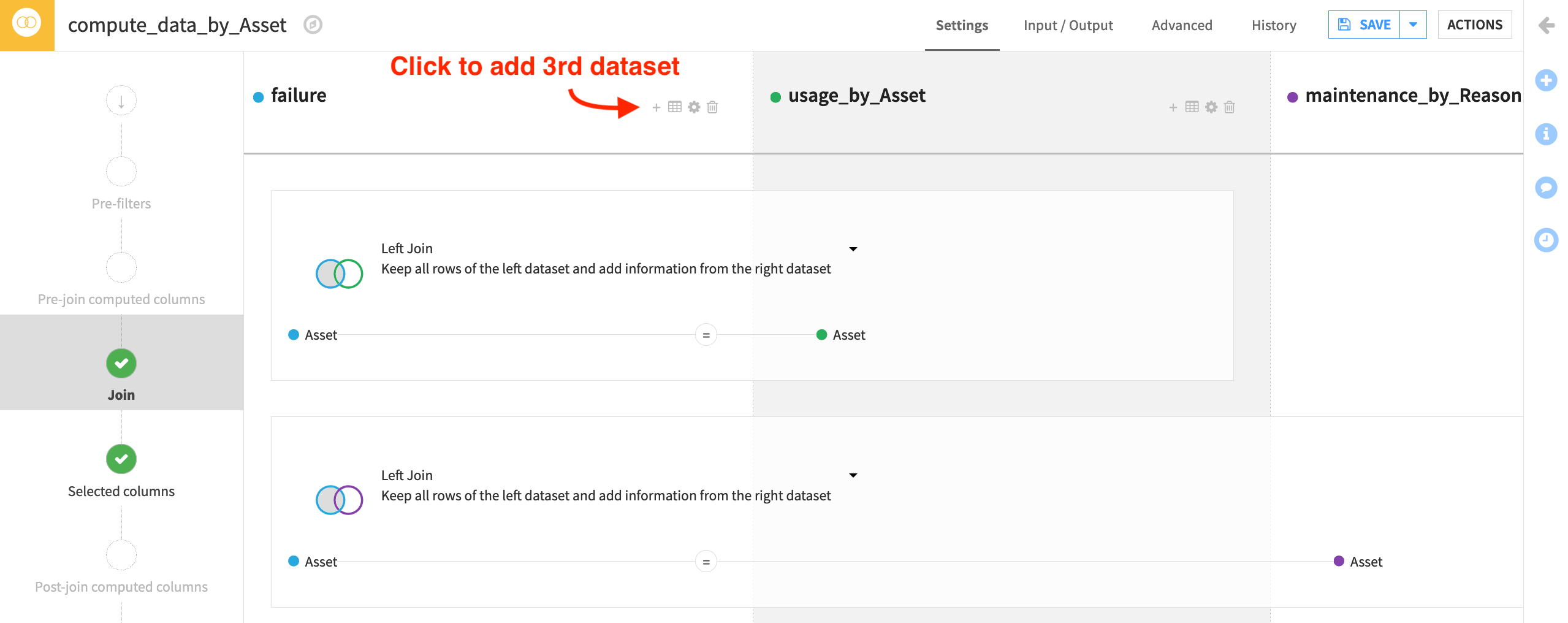
Name the output data_by_Asset, and click Create Recipe.
Add a third dataset maintenance_by_Reason to join to failure.
Both joins should be Left Joins. Asset should be the joining key in all cases.
Run the recipe, and confirm the output has 21 columns.

Note

To learn more on the Join recipe, see the following articles:

The data_by_Asset dataset now holds information from maintenance and usage, labelled by failures. Congratulations, great work!

Generate features#

Before making any models with the joined dataset, let’s create a few more features that may be useful in predicting failure outcomes.

Because we are still designing this workflow, we’ll create a sandbox environment that won’t create an output dataset—yet. By going into the Lab, we can test out such transformations, plus much more. Nothing is added back to the Flow until we are done testing!

Note

See the Concept | Visual analyses in the Lab and Tutorial | Visual analyses in the Lab articles to learn how steps in an analytics workflow can move from the Lab to the Flow.

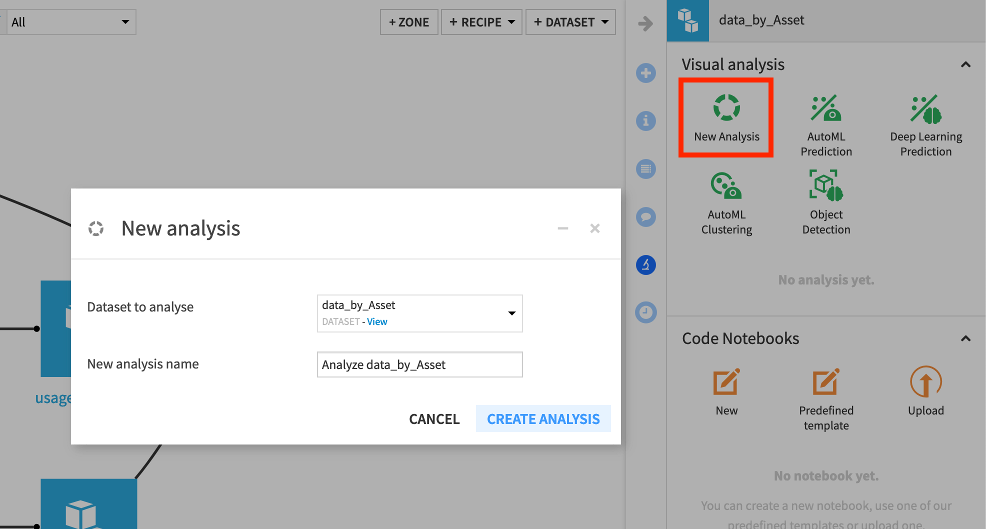
With the data_by_Asset dataset selected, navigate to the Lab in the right panel.
Create a New Analysis, and accept the default name Analyze data_by_Asset.

In the Script tab, which looks very similar to a Prepare recipe, let’s first use the “Rename columns” processor to rename the following 5 columns.

Old name	New name
count	times_measured
Time_min	age_initial
Time_max	age_last_known
Use_min	distance_initial
Use_max	distance_last_known

Create two new features with the Formula processor.
- distance from the expression, distance_last_known - distance_initial
- time_in_service from the expression, age_last_known - age_initial
Use the Fill empty cells with fixed value processor to replace empty values with 0 in columns representing reasons. The regular expression ^R.*_Quantity_sum$ is handy here.

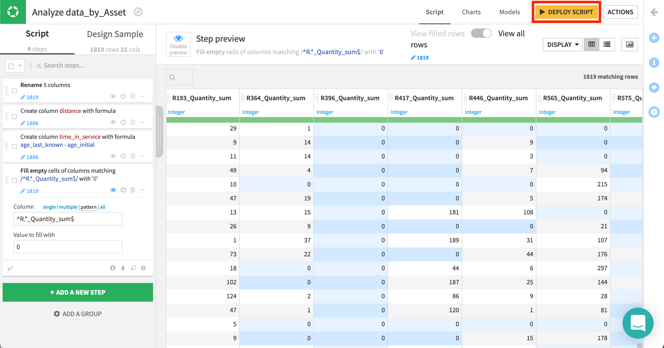
Once we’re satisfied with these features, we can deploy the script of the visual analysis as a Prepare recipe so all collaborators can see these data preparation steps in the Flow.

From the Script tab of the visual analysis, click the yellow Deploy Script button at the top right.
Accept the default output name, and click Deploy.
Then click to Run the Prepare recipe.

Note

Here we’ve taken the approach of deploying the Lab script to the Flow as a Prepare recipe. It’s also possible though to keep these data preparation steps within the visual analysis as part of the model object (which we’ll see). This can be helpful in some situations, such as deploying model as prediction endpoints.

Create the training & scoring datasets#

Before training models, we need to split the data. We will use the Split recipe to create two separate datasets from the merged and prepared dataset:

a training dataset will contain labels for whether or not there was a failure event on an asset. We’ll use it to train a predictive model.
a scoring dataset will contain no data on failures, i.e., unlabelled, so we’ll use it to predict whether or not these assets have a high probability of failure.

Here are the detailed steps:

From the data_by_Asset_prepared dataset, initiate a Split recipe.
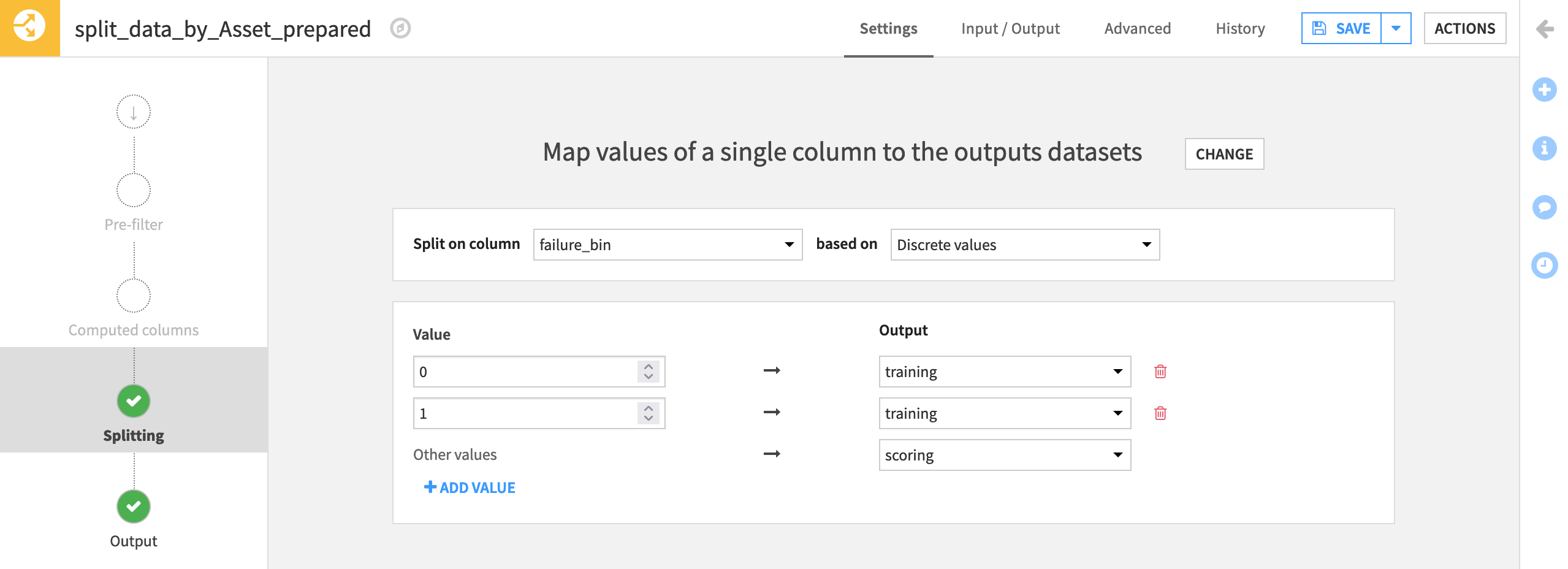
Add two output datasets, named training and scoring, selecting Create Dataset each time. Then Create Recipe.
At the Splitting step, choose to Map values of a single column.
Then choose failure_bin as the column to split on discrete values.
Assign values of 0 and 1 to the training set, and all “Other values” to the scoring set. (From the Analyze tool, we can see that these are the only possible values).
Run the recipe, and confirm the training dataset has 1,624 rows, and the scoring dataset has 195.

Create the prediction model#

Now that we have a dataset ready on which to train models, let’s use machine learning to predict car breakdown.

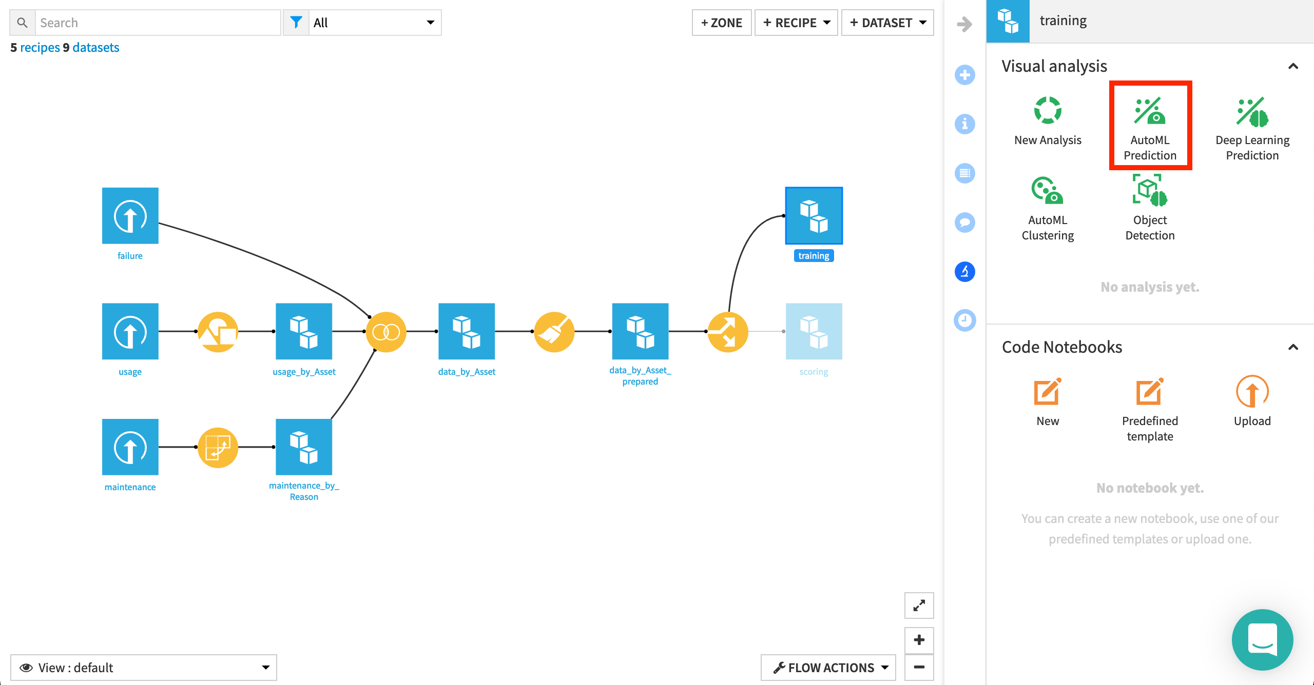
With the training dataset selected, click on AutoML Prediction in the Lab of the right panel.
Choose failure_bin as the target variable.

Note

Our goal is to predict a target variable (including labels), given a set of input features, and so we know this is a supervised learning problem, as opposed to clustering, or object detection for example.

You can learn more about this process in the Machine Learning Basics course.

Once we have picked the type of machine learning problem and target variable, we can choose between various kinds of AutoML or Export modes.

Leave the default Quick Prototypes, and click Create.
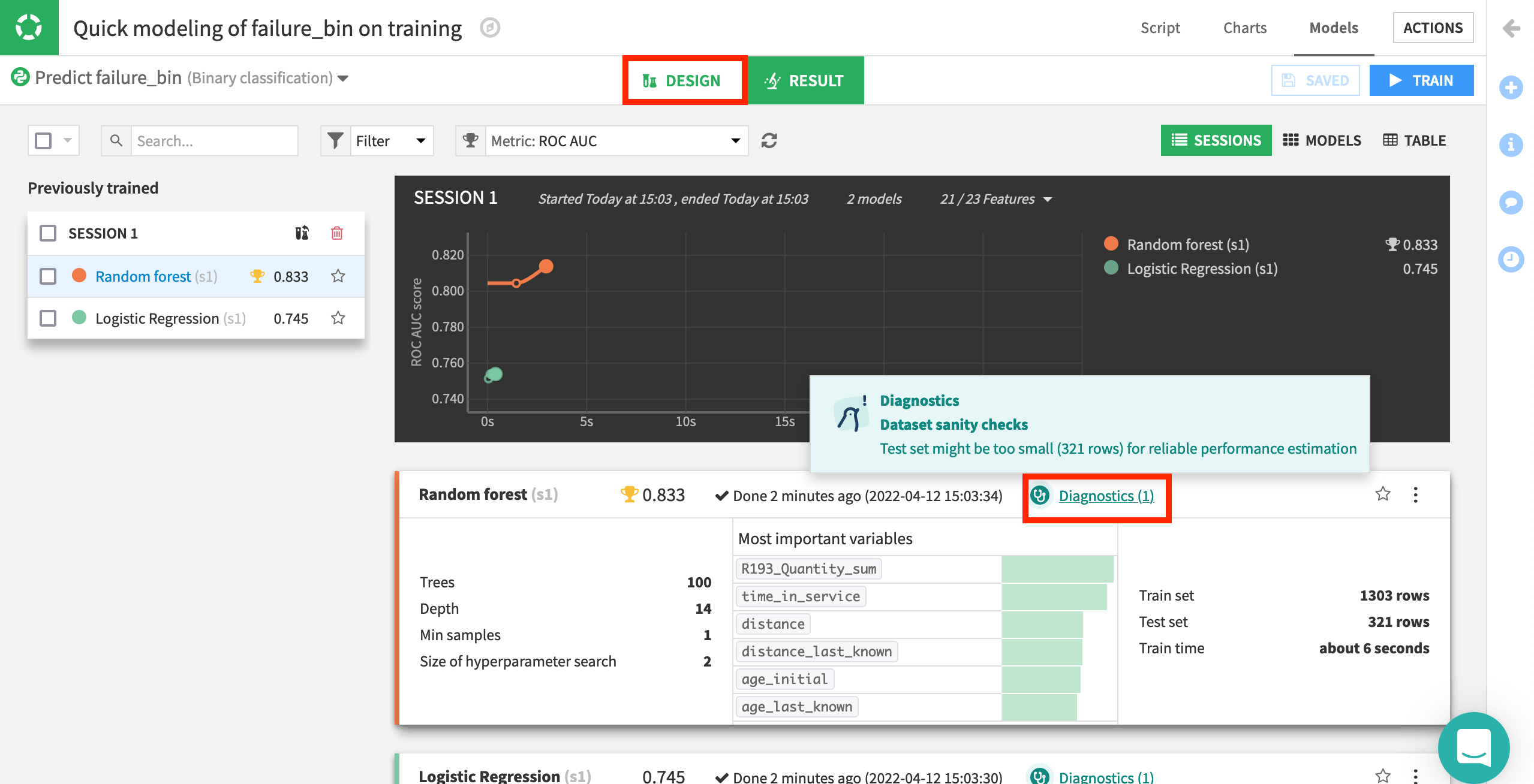
Click Train to build models using the default settings and algorithms, and wait for the results of the first training session.

Note

In the Results tab, you’ll notice each model has one diagnostic warning. This is Dataiku’s way of alerting us to potential machine learning problems—in this case, a dataset sanity check drawing attention to our small test set. For our purposes, we can ignore the warning. You can learn more about ML diagnostics in the reference documentation.

Once we have the results of some initial models, we can return to the Design tab to adjust all settings and train more models in additional settings if we wish.

Click on the Design tab to view the settings used to train the models in the first session.
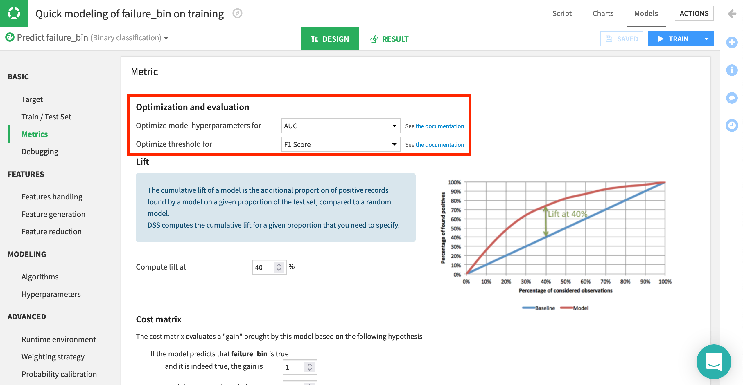
Navigate to the Basic > Metrics page from the left panel.

Here, we can define how we want model selection to occur. With these default settings, the platform optimizes for AUC (Area Under the Curve). That is, it picks the model with the best AUC, while the threshold (or probability cut-off) is selected to give the best F1 score. Similarly, feature engineering can also be tailored as needed, from which/how features are used, as well as options for dimension reduction.

Another important setting is the type of algorithms with which to model the data.

Navigate to Modeling > Algorithms.

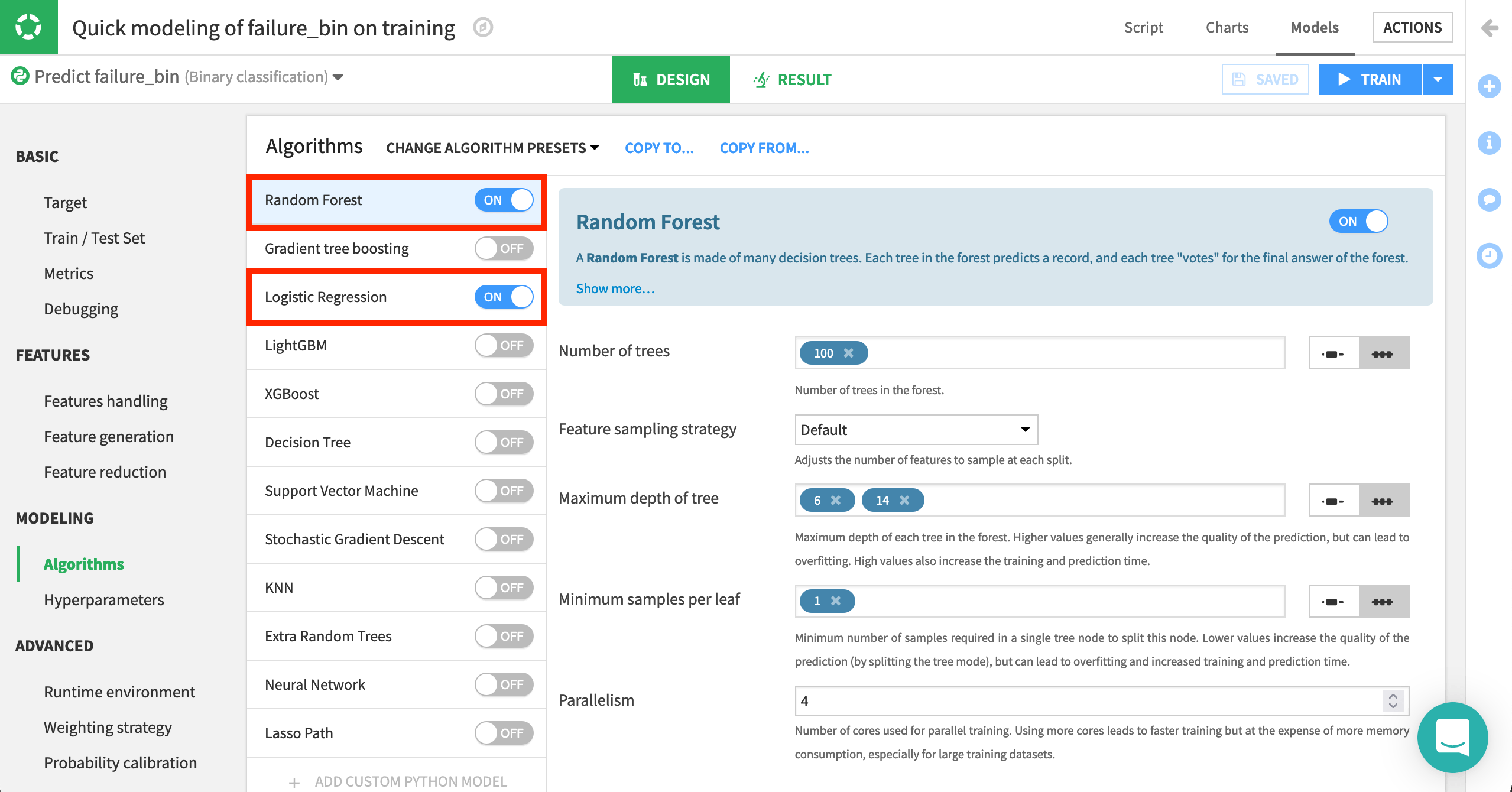
Here, we can select which native or custom algorithms to use for model training. In addition, we can define hyperparameters for each of them. For now, we’ll continue using two machine learning algorithms: Logistic Regression and Random Forest. They come from two classes of algorithms popular for these kinds of problems, linear and tree-based respectively.

Understand the model#

When satisfied with the design of the model, return to the Results tab.

Dataiku provides model metrics auto-magically! For example, we can compare how models performed against each other. By default, the AUC is graphed for each model. By that metric, random forest has performed better than logistic regression.

Switch from the Sessions view to the Table view to see a side-by-side comparison of model performance across a number of metrics.

Note

For more detail, we could also create a model comparison.

In this case, random forest has performed better across a number of different metrics. Let’s explore this model in greater detail.

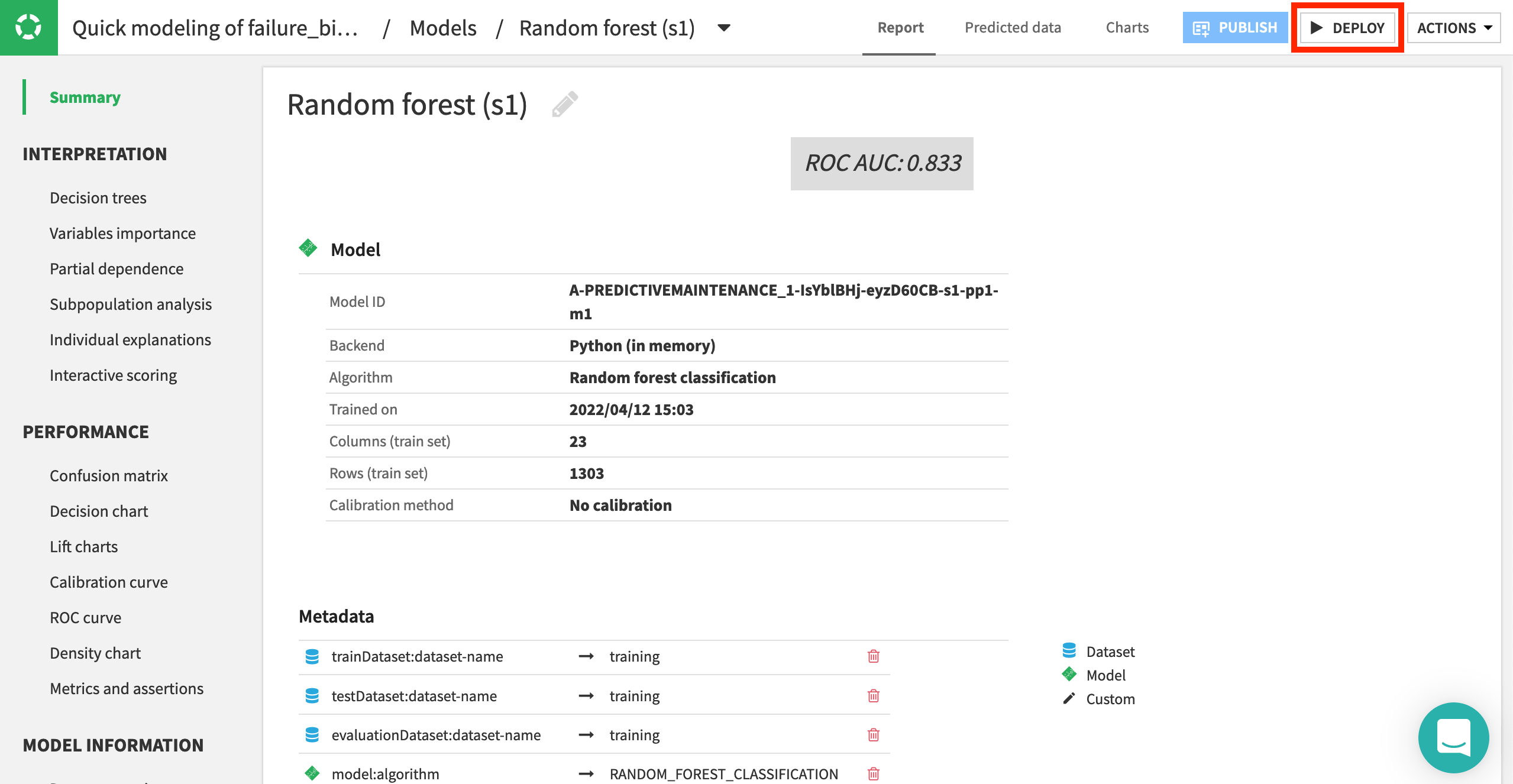
Click on the name of the model to view a more detailed report into the model’s interpretation, performance, and training information.

Note

Feel free to explore any of these panes to learn more about the model at hand.

You can learn more about prediction results in the reference documentation.

Score unlabeled data#

Let’s use this random forest model to generate predictions on the unlabelled scoring dataset. Remember, the goal is to assign the probability of a car’s failure.

From the Result tab of the visual analysis, click on the random forest model (the best performing model)—if not already open.
Click the Deploy button near the top right.
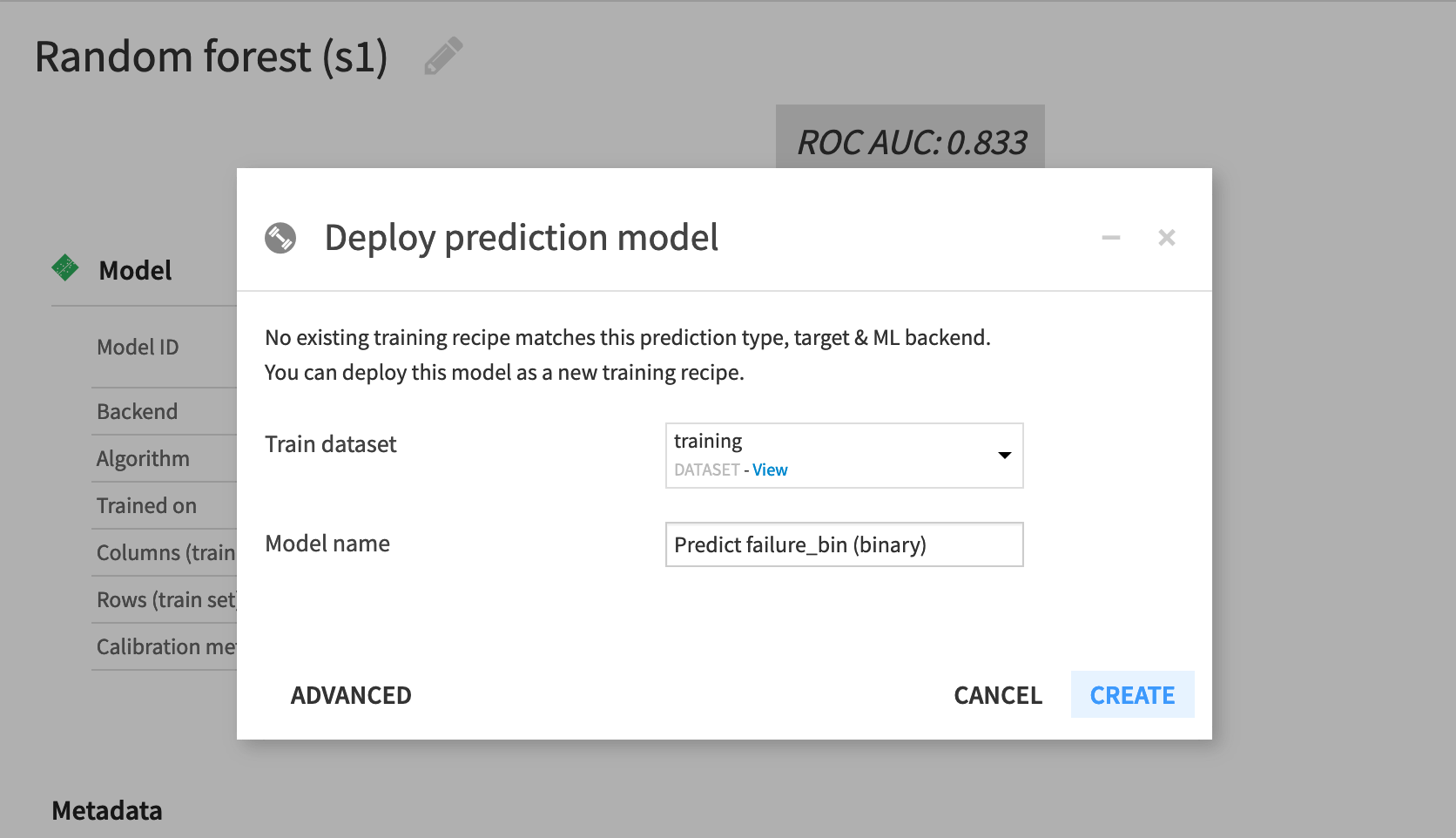
training dataset should already be selected as the Train dataset in the “Deploy prediction model” window.
Accept the default model name, and click Create.

Now back in the Flow, you can see the training recipe and model object. Let’s now use the model to score the unlabelled data!

In the Flow, select the model we just created. Initiate a Score recipe from the right sidebar.
Select scoring as the input dataset.
Predict failure_bin (binary) should already be the prediction model.
Name the output dataset scored.
Create and run the recipe with the default settings.

Note

There are multiple ways to score models in Dataiku. For example, in the Flow, if selecting a model first, you can use a Score recipe (if it’s a prediction model) or an Apply model (if it’s a cluster model) on a dataset of your choice. If selecting a dataset first, you can use a Predict or Cluster recipe with an appropriate model of your choice.

Compare the schema of the scoring and scored datasets. (It’s easiest to do this from the Schema tab of the right panel in the Flow).

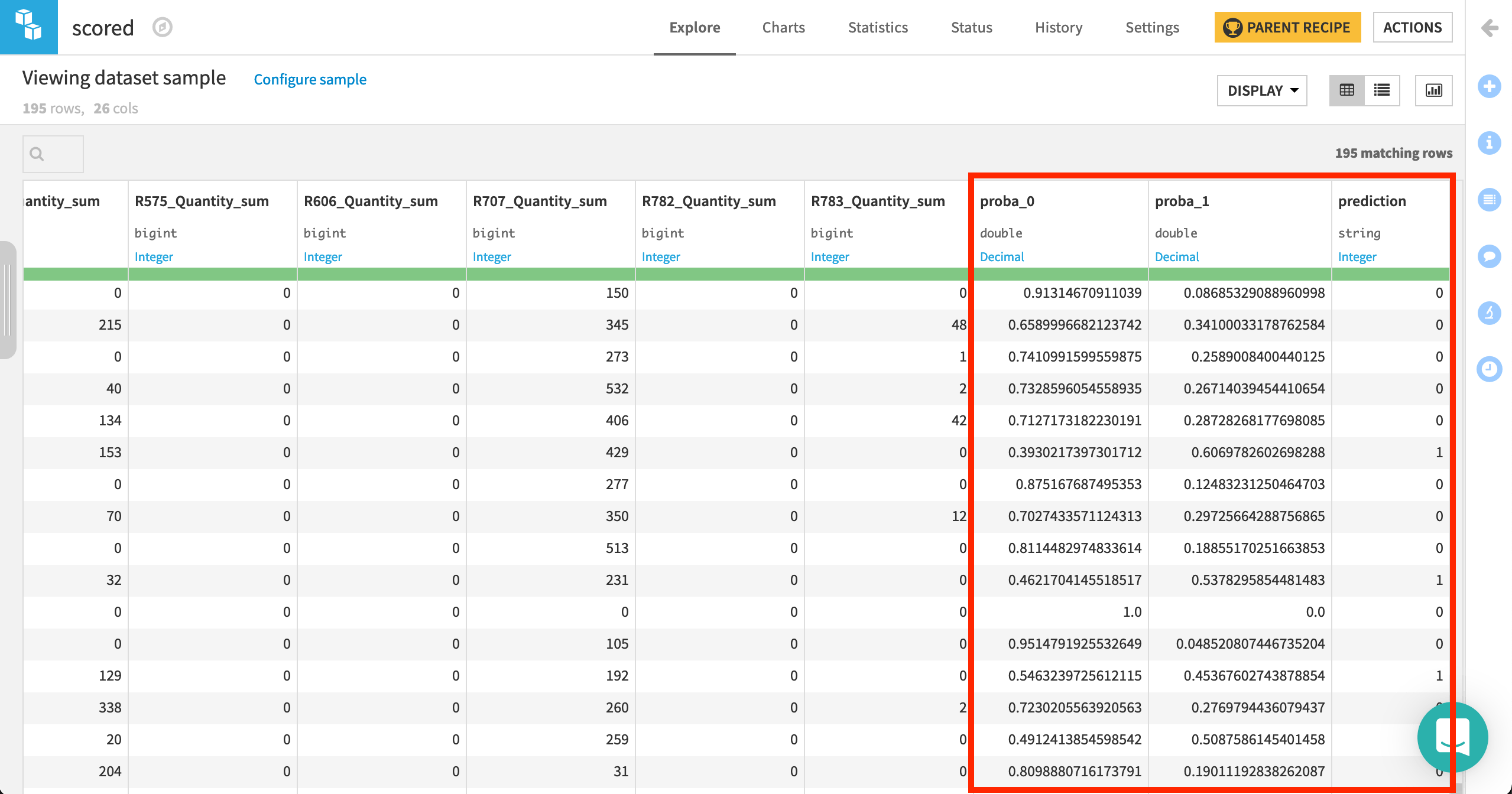
Then, the prepared scoring dataset is passed to the model, where three new columns are added:
- proba_1: probability of failure
- proba_0: probability of non-failure (1 - proba_1)
- prediction: model prediction of failure or not (based on probability threshold)

Identify high risk assets#

Let’s now go one step further, and use the probabilities generated by the model to one identify two tiers of risk.

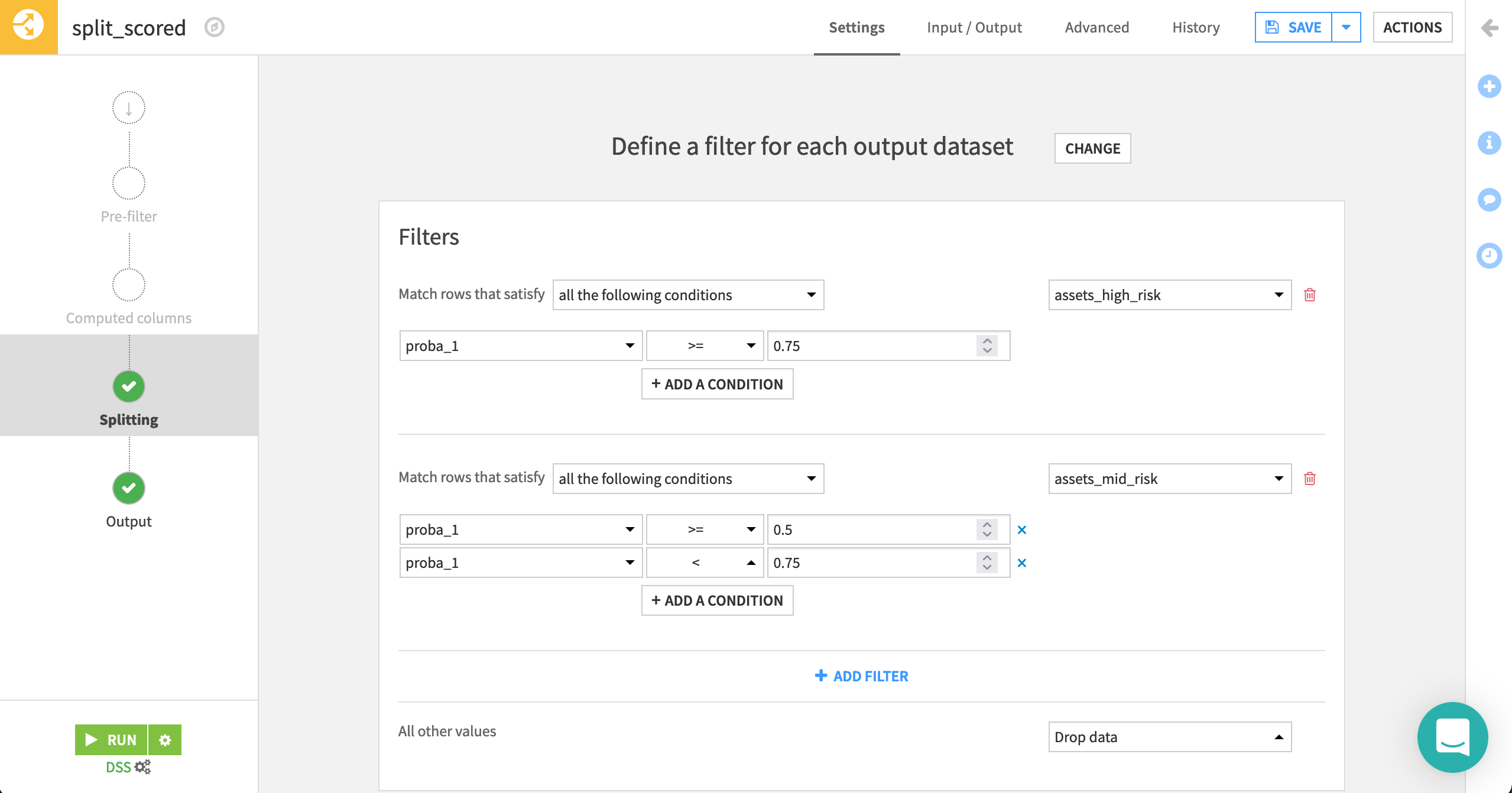
Add a Split recipe to the scored dataset with two outputs: assets_high_risk and assets_mid_risk.
Choose Define filters as the splitting method.
- Rows matching the condition proba_1 >= 0.75 should be sent to the assets_high_risk dataset.
- Rows matching the two conditions proba_1 >= 0.5 and proba_1 < 0.75 should be sent to the assets_mid_risk dataset.
- All other values should be dropped.
Run the recipe.

Automate the Flow#

Our Flow now has two final outputs: a dataset identifying the highest risk assets in need of maintenance and another dataset of assets still at risk, but of a somewhat lower urgency.

Imagine that new data must travel through this pipeline on a daily basis. We need a way to automate building this Flow every day to take into account the new data collected by sensors during the day. Scenarios are the way to achieve this in Dataiku.

From the Jobs menu in the top navigation bar, click on Scenarios.
On the Scenarios page, click + New Scenario or + Create Your First Scenario.
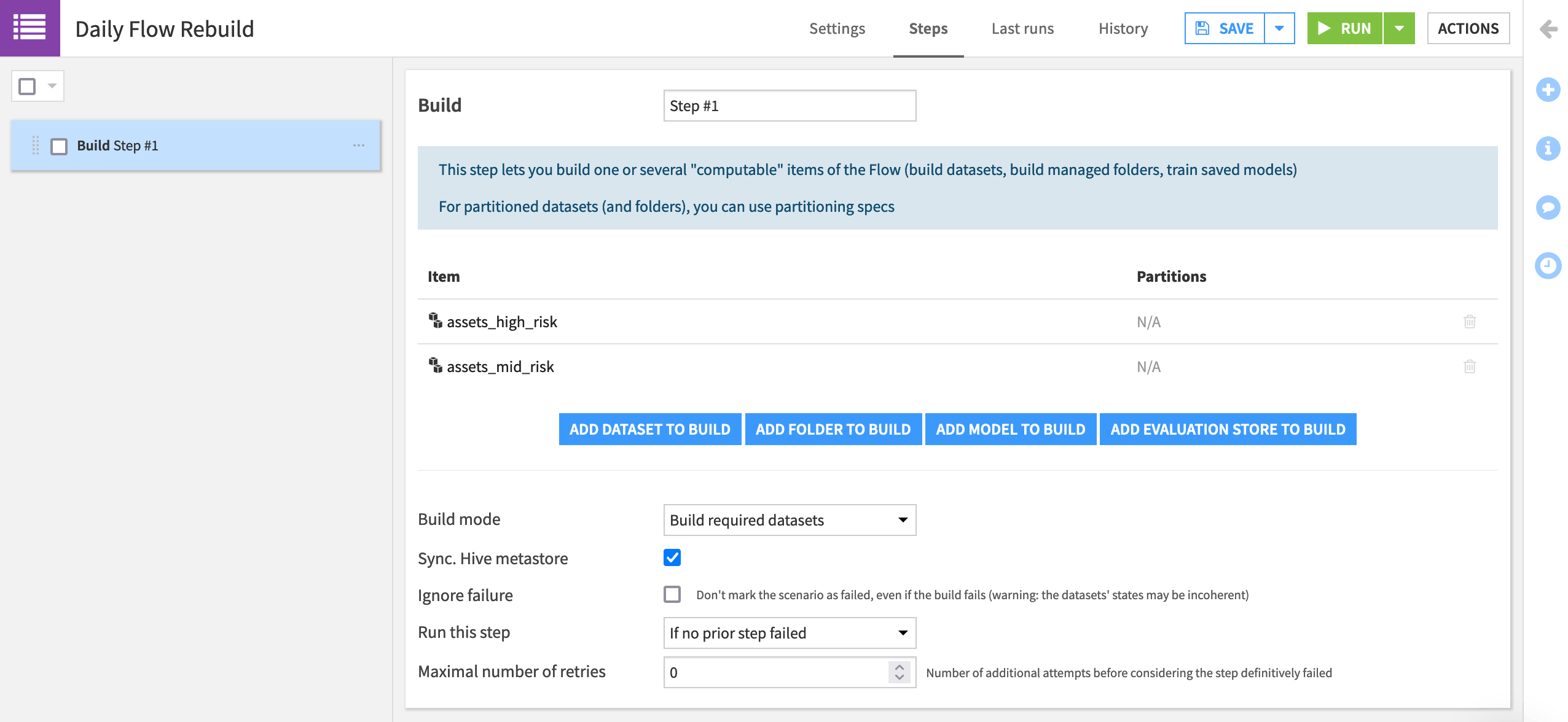
Name it Daily Flow Rebuild, and click Create.
In the Steps tab of the scenario, add a Build / Train step.
Add assets_high_risk and assets_mid_risk as the datasets to build.
The “Build mode” is already set to build required datasets, and so we only need to specify the final desired output, and Dataiku will determine the best way to do that.
Save your work.

Now we know what action the scenario will complete, but when should it run?

Navigate to the Settings tab of the scenario.
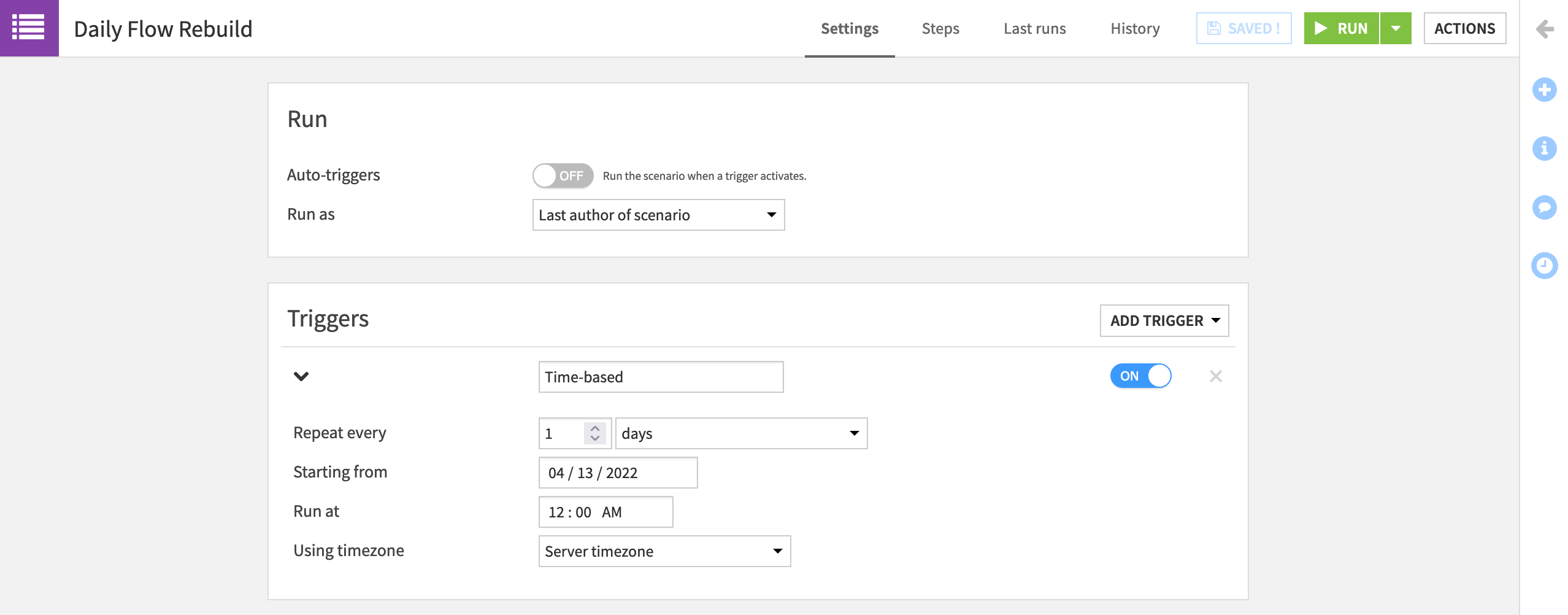
Add a time-based trigger.
Configure the scenario to repeat every 1 day at midnight.
Save your work.

Now let’s test it instead of waiting for the trigger to activate!

Click the green Run button to manually trigger the scenario.
Navigate to the “Last Runs” tab to view its progress.

What happened here? If you click on the job, you’ll see that there actually was nothing for Dataiku to do. With the Build mode set to “Build required datasets”, and no new data present in the pipeline, Dataiku did not need to take any action to give us the requested output.

Feel free to adjust the Build mode of the Build/Train step in the scenario to “Force rebuild” just to see how it would run through building the pipeline for the scenario.

Note

The scenario shown here is the absolute most basic version. For a more in-depth look, see the Data Quality & Automation course.

Deploy the project to production (optional)#

Now that a scenario has been created to automate the rebuild of the Flow and score new assets every day, it is time to batch deploy the whole project to a dedicated production environment, the Automation node.

Warning

In order to complete this last section, you’ll need to satisfy a few additional requirements:

a Business or Enterprise license
a Design node connected to an Automation node and deployment infrastructure
a user profile belonging to a group with access to the deployment infrastructure

From the More Option (…) menu in the top navigation bar, choose Bundles.
Click + New Bundle or + Create Your First Bundle.
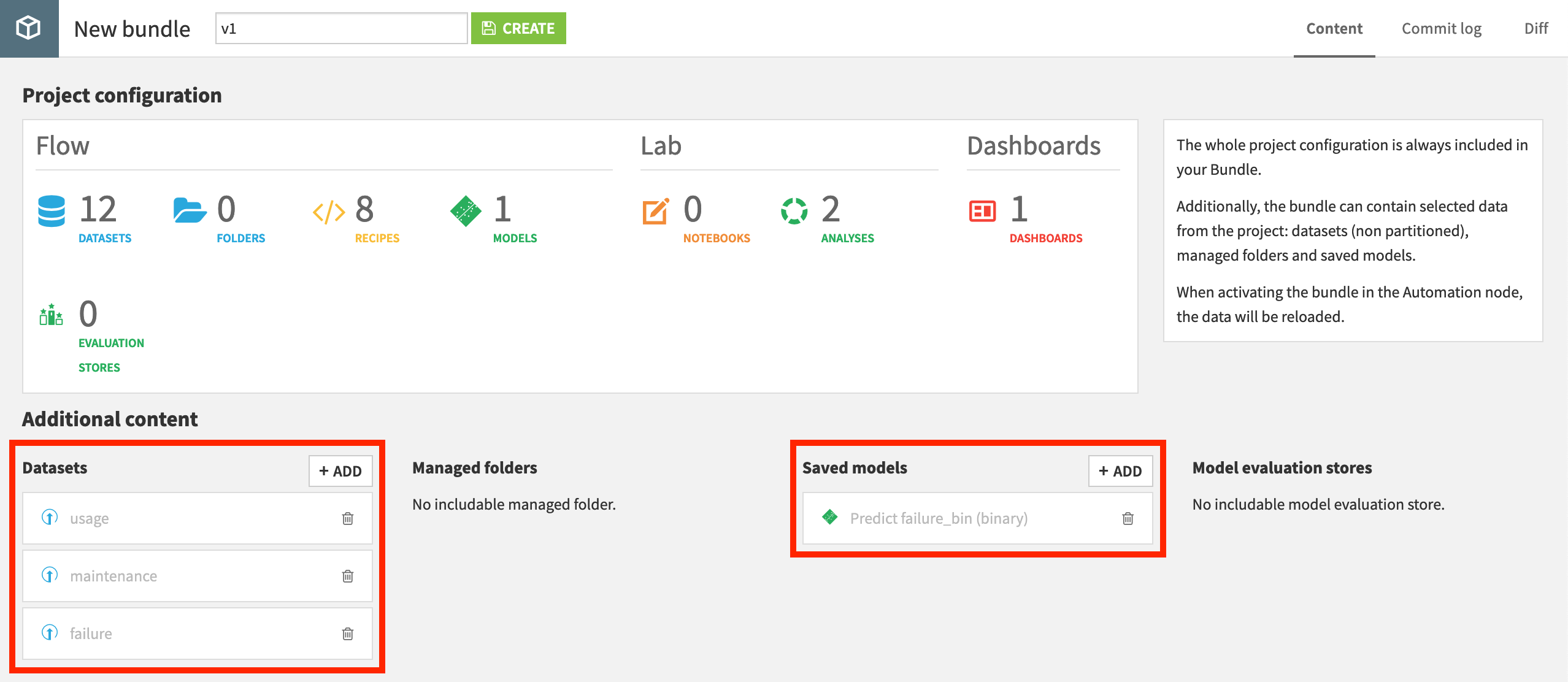
Since our data in this case is not coming from an external database connection, add the three uploaded datasets: failure, maintenance, and usage.
Also, add the saved model to be included in the bundle.
Name the bundle v1, and click Create.

Now that we have a bundle, we can publish it on the Deployer, and from there deploy it to the Automation node.

From the Bundles page, click on the v1 bundle, and click Publish on Deployer.
Confirm that you want to Publish on Deployer.
Open the bundle in the Deployer.
Now in the Deployer, click Deploy to actually create the deployment.
Choose an available target infrastructure, and click Create.
Finally, click Deploy and Activate.

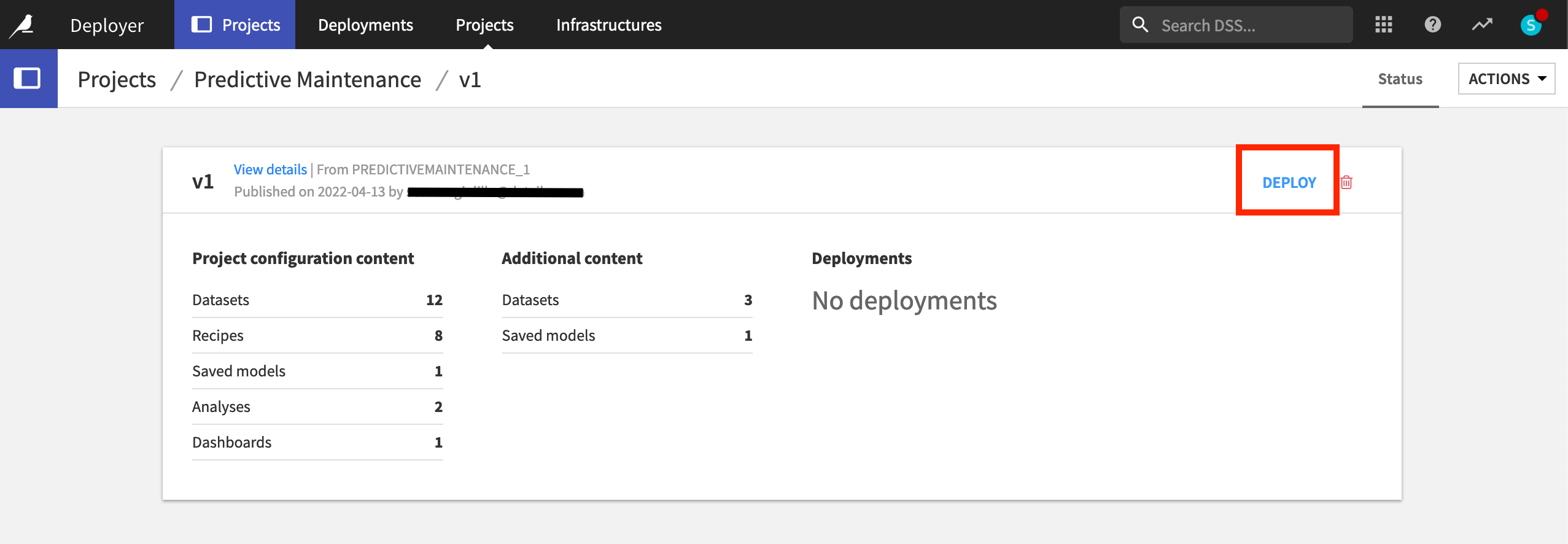
Once the deployment has been created, we can view the bundle running on the Automation node.

From the Status tab of the new deployment, click on the link for the Automation project.
Once on the Automation node, confirm in the project homepage that it’s running the v1 bundle.
Then go to the Scenario tab, and turn on the scenario’s auto-trigger.
Although it has no new data to consume, Run the scenario to confirm it is now running in a production environment separate from the Design node.

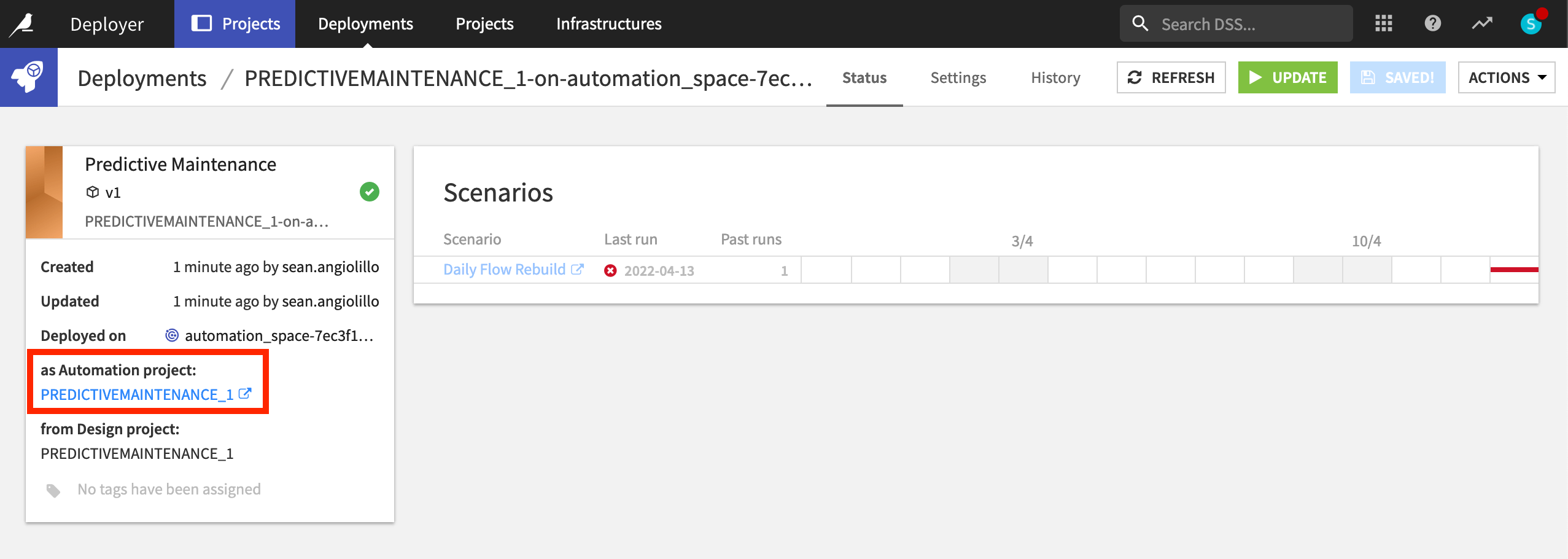
Voilà! You now have a predictive maintenance project deployed in production!

Note

The process for batch deployment is covered in much greater detail in the Project Deployment.

Wrap-up#

And that’s a wrap!

The goal here was to build an end-to-end data product to predict car failures from a workflow entirely in Dataiku. Hopefully, this data product will help the company better identify car failures before they happen!

Once we have a single working model built, we could try to go further to improve the accuracy of this predictive workflow in a number of ways, such as:

Adding more features to the model by combining information in datasets in more ways
Trying different algorithms and hyper-parameter settings

Visit the Dataiku Academy for more courses and learning paths to increase your proficiency with Dataiku!